

Appendix Stiffness matrix for 2D beam element

5. Appendix Stiffness matrix for 2D beam element#

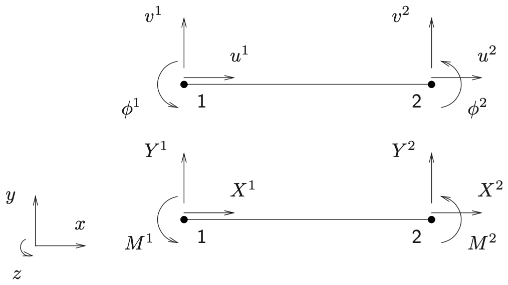
In Fig. 5.16 below a two-dimensional beam element is drawn, where the beam axis is oriented according to the \(x\)-axis.
_images/Mentat-fig30.png

Fig. 5.16 Degrees of freedom \(u\), \(v\), \(\varphi\) and their conjugate nodal forces \(X\), \(Y\), \(M\) for a prismatic beam element between nodes 1 and 2, shown in the local \(x\)–\(y\) plane with the global \(z\) axis pointing out of the page.#

The stiffness matrix of this beam element describes the relation between the nodal degrees of freedom and the nodal forces and momenta. By making use of the mechanical beam equations the stiffness matrix can be created:

\[\begin{split} \begin{bmatrix} X^{1}\\[2pt] Y^{1}\\[2pt] M^{1}\\[2pt] X^{2}\\[2pt] Y^{2}\\[2pt] M^{2} \end{bmatrix} \;=\; \begin{bmatrix} \dfrac{EA_{0}}{l_{0}} & 0 & 0 & -\dfrac{EA_{0}}{l_{0}} & 0 & 0 \\[6pt] 0 & \dfrac{12EI}{l_{0}^{3}} & \dfrac{6EI}{l_{0}^{2}} & 0 & -\dfrac{12EI}{l_{0}^{3}} & \dfrac{6EI}{l_{0}^{2}} \\[6pt] 0 & \dfrac{6EI}{l_{0}^{2}} & \dfrac{4EI}{l_{0}} & 0 & -\dfrac{6EI}{l_{0}^{2}} & \dfrac{2EI}{l_{0}} \\[6pt] -\dfrac{EA_{0}}{l_{0}} & 0 & 0 & \dfrac{EA_{0}}{l_{0}} & 0 & 0 \\[6pt] 0 & -\dfrac{12EI}{l_{0}^{3}} & -\dfrac{6EI}{l_{0}^{2}} & 0 & \dfrac{12EI}{l_{0}^{3}} & -\dfrac{6EI}{l_{0}^{2}} \\[6pt] 0 & \dfrac{6EI}{l_{0}^{2}} & \dfrac{2EI}{l_{0}} & 0 & -\dfrac{6EI}{l_{0}^{2}} & \dfrac{4EI}{l_{0}} \end{bmatrix} \begin{bmatrix} u^{1}\\[2pt] v^{1}\\[2pt] \varphi^{1}\\[2pt] u^{2}\\[2pt] v^{2}\\[2pt] \varphi^{2} \end{bmatrix} \end{split}\]

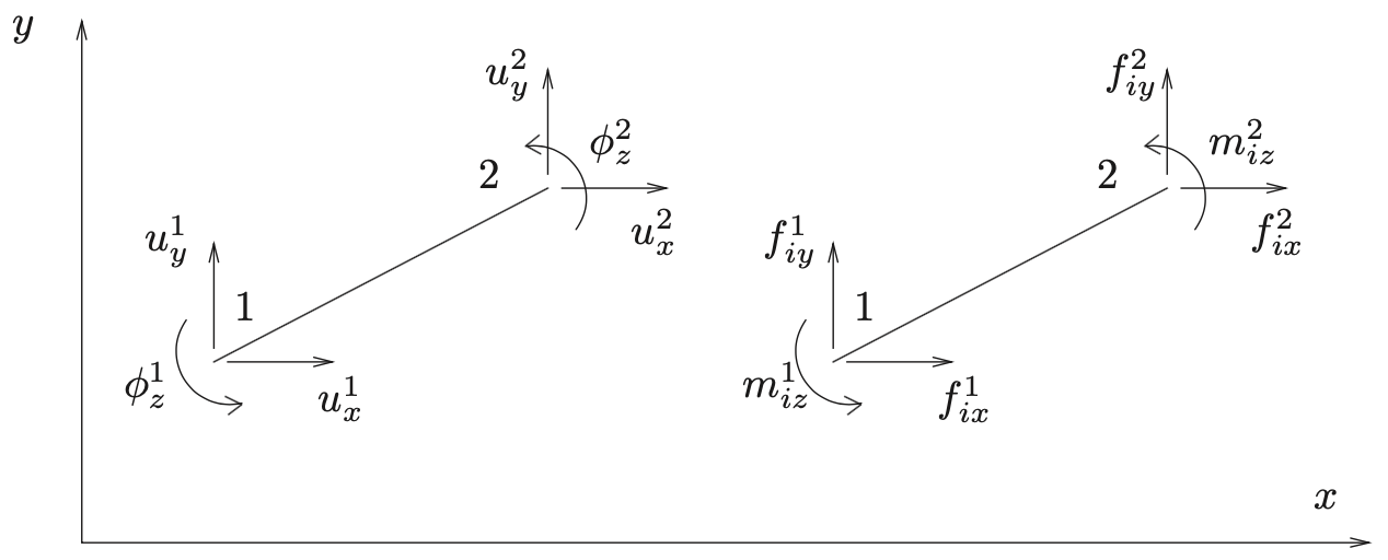
In the general case, the beam axis makes an angle (say \(\alpha\)) with the x-axis, as shown in Fig. 5.17 below.
_images/Mentat-fig31.png

Fig. 5.17 Local \(x\)–\(y\) axis definition and sign convention for a plane-frame (2-D beam) element. Nodal translations \((u_x,u_y)\) and rotation \(\varphi_z\) are given at nodes 1 and 2, together with the corresponding internal forces \((f_{ix},f_{iy})\) and bending moment \(m_{iz}\).#

The six degrees of freedom and the six forced are stored in columns:

\[ \col{u}^e = [u_x^1\; u_y^1 \; \phi_z^1 \; u_x^2 \; u_y^2 \phi_z^2]^T \quad ; \quad \coli{f}^{\;e} = [f_{ix}^1\; f_{ix}\; f_{iy}^1 \; m_{iz}^1 \; f_{ix}^2 \; f_{iy}^2 \; m_{i7}^2 ]^T \]

The relation between \(\col{u}^e\) and \(\coli{f}^{\;e}\) is described with the element stiffness matrix \(\mat{K}^e\). This is obtained from the above matrix \(\matl{K}^e\) by a transformation that takes into account the rotation. The rotation matrix \(\mat{R}\) is a function of the angle \(\alpha\) and reads:

\[\begin{split} \mat{R} \;=\; \begin{bmatrix} c & s & 0 & 0 & 0 & 0 \\[2pt] -s & c & 0 & 0 & 0 & 0 \\[2pt] 0 & 0 & 1 & 0 & 0 & 0 \\[2pt] 0 & 0 & 0 & c & s & 0 \\[2pt] 0 & 0 & 0 & -s & c & 0 \\[2pt] 0 & 0 & 0 & 0 & 0 & 1 \end{bmatrix} \qquad;\qquad c=\cos(\alpha)\,,\;\; s=\sin(\alpha) \end{split}\]

The transformation is taking place as follows:

\[ \mat{K}^e = \mat{R}^T \matl{K}^e \mat{R} \]