
4. Constitutive equations (stress-strain relations)#
Book: Introduction Chapter 3, Sections 3.1 to 3.3.
4.1. Relations between stress and strain#
Relations between stress and strain are also called constitutive relations.
Consider an infinitesimally small rectangular block of material cut out of a loaded structure, where edges of the block are aligned with the axes of a Cartesian \((x,y,z)\)-coordinate system. Next, consider a triaxial state of stress with normal stresses \(\sigma_x\), \(\sigma_y\) and \(\sigma_z\) on the faces of the block. If \(\sigma_x = \sigma_y = \sigma_z = \sigma_\text{H}\) it is called a hydrostatic state of stress. If \(\sigma_\text{H}\) is negative, such as often is the case for fluids, \(-\sigma_\text{H}\) is called a hydrostatic pressure.
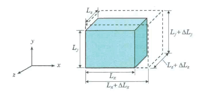
Fig. 4.1 Loaded structure with edges aligned towards cartesian coordinate system.#
Assuming the lengths of the edges are \(L_x\), \(L_y\) and \(L_z\) in the unloaded state (as depicted in Fig. 4.1), we have three strains associated with the hydrostatic state of stress:
Under load, the deformed volume becomes
Now we define the volumetric strain or dilatation as follows:
If \(e_x \ll 1\), \(e_y \ll 1\) and \(e_z \ll 1\) we have the following approximation: \(e_\text{vol} = e_x + e_y + e_z\).
For an isotropic material, where the properties are the same for all directions, we have
Note, that many materials such as wood, reinforced concrete and fibre-reinforced polymers are anisotropic, i.e.\(\,\) the properties are direction dependent.
The relation between \(\sigma_\text{H}\) and \(e_\text{vol}\) is linear for most materials (see Figure 3.3).
4.2. Hooke’s law#
For many materials there is a linear relation between the tensile stress and strain in a uniaxial tensile test. This property can be written as follows: \(\sigma = Ee\). This is called Hooke’s law. The coefficient \(E\) is the modulus of elasticity or Young’s modulus of the material.
Consider a rectangular bar of material having an initial length of \(L_0\) as depicted in Fig. 4.2, initial thickness \(d_0\) and initial width \(b_0\) subjected to a uniaxial stress \(\sigma\). Under load the dimensions of bar become \(L_0 + \Delta L\), \(d_0 - \Delta d\) en \(b_0 - \Delta b\). The axial strain becomes \(\displaystyle e_\text{L} = \Delta L/L_0 \), whereas the strain in depth and width directions become \( \displaystyle e_\text{d} = -\Delta d/d_0 \) and \( \displaystyle e_\text{b} = -\Delta b/b_0 \), respectively.
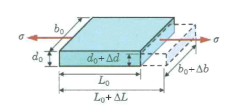
Fig. 4.2 Rectangular box sunjected to a unaxial stress \(\sigma\).#
Warning
Here the authors of the book use an inconsistent definition for the changes in size. It is almost universally accepted that a change is positive if a quantitive increases and negative if it decreases However, here \(\Delta L\), \(\Delta d\) and \(\Delta b\) are defined such that the signs are the same for the most common case. However, it is much better to adhere to the usual definition and define:
and use the same strain definition in the three directions:
The conclusions do not change. Only the expressions for the strains are different.
From experiments we find for linear elastic material behaviour that the strains in perpendicular direction are proportional to the axial strain: \(e_\text{d} = e_\text{b} = -\nu e_\text{L}\). The parameter \(\nu\) is a material constant and is called Poisson’s ratio. The value of \(\nu\) is usually between 0 and \(0.5\). For most metals \(\nu=0.3\) and for rubbery materials the value of \(\nu\) is close to \(0.5\).
For the triaxial state of stress as depicted in Figure~3.1, the corresponding triaxial state of strain is given by the following generalised Hooke’s law:
This state of strain is obtained by adding or superimposing the strains corresponding with the three stress components. The general principal of superposition states that:the total effect of a combination of loads is the sum of the effects of the individual loads separately. This principal is valid if there is a linear relation between stresses and strains, and strains due to the individual loads are small.
Apparent modulus of elasticity
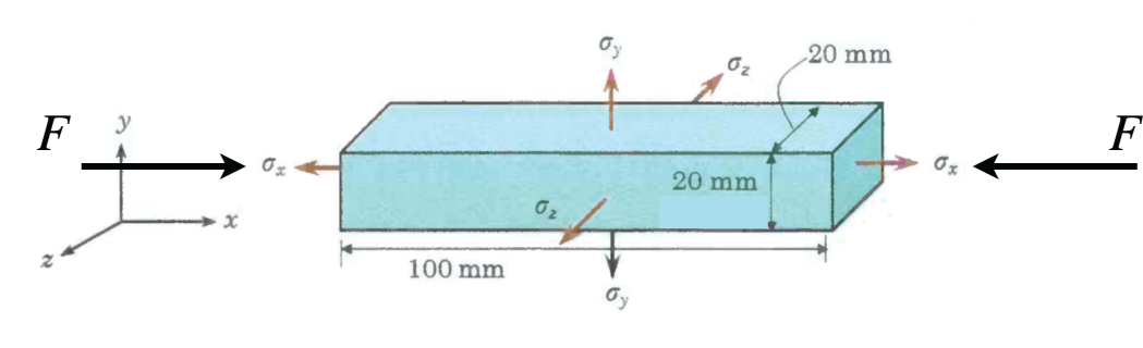
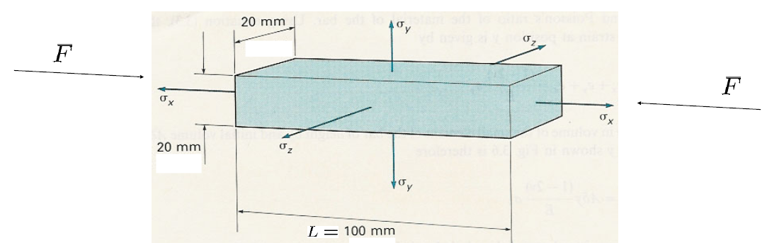
Fig. 4.3 Rectangular box experiencing normal stresses.#
The system depicted in Fig. 4.3 experiences two forces one on the \(\sigma_x\) and one on the \(- \sigma_x\) side. the lenght, width and height of the box are \(100\) mm, \(20\) mm and \(20\) mm repsectively. Find the change in lenght and the apperent modulus of elasticity for the system.
Solution
The bar is loaded only in the \(x\)-direction by an axial force \(F\) Its ends are free to move axially, but the faces perpendicular to \(y\) and \(z\) are constrained so that
and next to this we also know that
Since the lateral (\(y\) and \(z\)) stresses \(\sigma_y\) and \(\sigma_z\) are not zero in general, they must develop whatever value is needed to enforce \(\displaystyle e_y = e_z = 0 \). By symmetry we set
For an isotropic solid the small-strain Hooke’s law gives, in they y direction,
Using substitution of the earlier found relation for \(-p\) gives
Thus finally when solving for \(p\) we get
The next step is solving for \(e_x\) which is given by
where the earlier found relations for \(p\) are used again. This gives
with the relation \(\displaystyle e_x= \frac{\sigma_x}{E'}\) finally
For shear loading in the linear elastic regime, (Hooke’s law for shearing) is valid:
The constant \(G\) is called the shear modulus (of elasticity). The shear strain in one direction is not influenced by the shear loading in the directions normal to it.
For hydrostatic loading a linear relation is valid between the hydrostatic stress and the volumetric strain:
where \(K\) is called the bulkmodulus (of elasticity).
For a triaxial state of stress having normal stresses \(\sigma_x\), \(\sigma_y\) and \(\sigma_z\), the following relation can easily be derived from the generalised Hooke’s law:
For a hydrostatic state of of stress, i.e.\ \(\sigma_x = \sigma_y = \sigma_z = \sigma_\text{H} \), it follows that
This leads to \(\displaystyle E = 3K(1-2 \nu)\). For \(\nu=0.5\), we see that \(K=\infty\), assuming \(E\) is finite. This means that the material is incompressible.
In Chapter 9 it is derived that the shear modulus \(G\) can be expressed in the two material parameters \(E\) and \(\nu\) according to \(G=E/2(1+\nu)\). For realistic materials \(E\), \(K\) and \(G\) are always positive, which leads to \(-1 \leq \nu \leq 0.5\). In practice we have \(0\leq \nu \leq 0.5\).
4.3. Thermal strains#
Changes in temperature can cause strains. It is well-known, that for a large class of materials we have \(e_x = \alpha \Delta T\), \(e_y = \alpha \Delta T\) en \(e_z = \alpha \Delta T\), if the material is able to freely expand (no constraints). Here, \(\Delta T\) is the increase in temperature and \(\alpha\) is the coefficient of linear thermal expansion, for which we have \(\alpha\geq0\). In general, the coefficient \(\alpha\) depends on temperature, however in many cases it can be assumed to be constant for certain ranges of temperature.
The volumetric strain of a freely expanding material is given by
where \(\beta\) is the coefficient of volumetric thermal expansion.
Superposition of the strains due to mechanical loading and the thermal strains leads to:
Shear strains are not affected by changes in temperature, i.e.\(\,\) \(\tau = G \gamma\) is still valid here.
Change in volume of a block
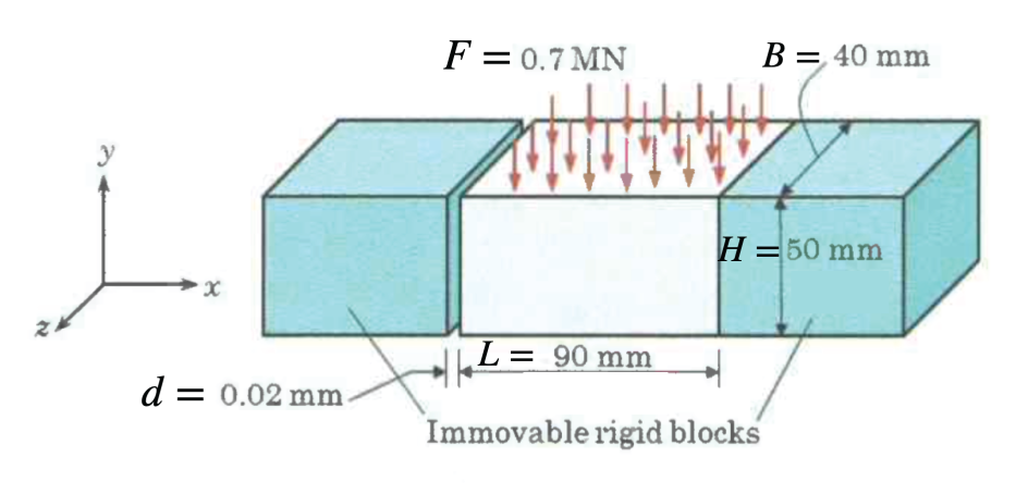
Fig. 4.4 thermally and mechanically constrained rectangular box.#
A thermo‐elastic, three-dimensional stress–strain problem in which a rectangular steel block is both thermally and mechanically constrained is concidered. The problem is depicted in Fig. 4.4. The steel specimen that is constrained has dimensions \(L= 90\) mm, \(B = 40\) mm (width), \(H = 50\) mm (height). Its ends sit against two immovable rigid blocks, but there is initially a small clearance \(d = 0.02\) mm between the specimen and the rigid stops.
The block is uniformly heated by \(\displaystyle \Delta T = 15 \ \rm ^{\circ}\rm C\). Simultaniously a total normal force \(\displaystyle F = 0.7 \rm MN\) is applied as a uniformly distributed presure on the top pace (\(y\)-direction).
The material properties of steel are given by \(\displaystyle E = 207 \rm GPa\), \(\displaystyle \nu = 0.30\) and \(\displaystyle \alpha = 11\times 10^{-6} \ \rm ^{\circ} \rm C^{-1}\).
Determine the uniformly distributed forces and the change in volume of the block.
Solution
the total strain in \(x\) is prescribed by the gap:
In equilibrium the only non-zero stress from the load \(F\) is
Steel expands freely by an amount \(\alpha \Delta T\) in every direction heated by \(\displaystyle \Delta T = 15 \ \rm ^{\circ}\rm C\). But here the rigid blocks resist the \(x\)–expansion, so a reaction stress \(\sigma_x\) develops. Thus \(e_x\) concists of a mechanical and a therma strain
Solving with previous relations gives
Since
we need to compute \(e_{\rm vol}\). This is done via hookes law and gives
Thus
represents the change in volume due to the thermal and mechanical constrains.
Note
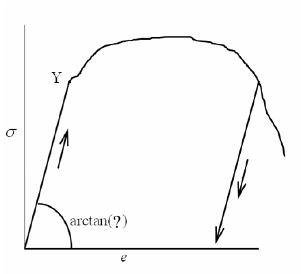
Section 3.3 of the book is not part of the exam. In general, we can say that material behaviour is time-dependent, showing viscoelastic, viscoplastic or viscoelastic-plastic response. Plastic response here refers to material behaviour showing a permanent deformation after fully unloading. These non-elastic constitutive relations will be a subject of courses later in the curriculum.
4.4. Additional Video#
This video by The Efficient Engineer gives another perspective on the relationship between stress and strain by introducing the concept of Poisson’s Ratio. This video is non-mandatory and is purely to give a different perspective on the topic.