
11. Thin-walled cylinders and spheres loaded with internal pressure. Buckling of struts and columns#
Book: Section 2.2 excluding 2.2.3. Introduction to Chapter 8, Sections 8.1, 8.2 1, Intro of 8.3, 8.3.1 and 8.3.5, excluding the last paragraph before Example 8.7.The Euler buckling formula for struts and columns
11.1. Uniformly loaded thin shells.#
11.2. Thin-walled cylinder#
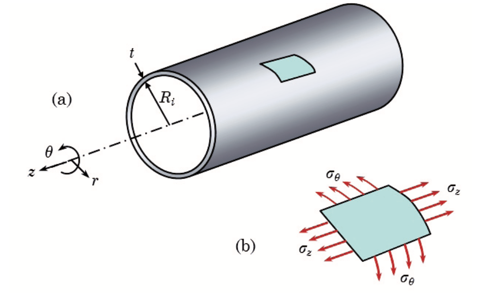
Fig. 11.1 Long cylinder with a circular cross section with internal radius \(R_\text{i}\) and a constant thickness \(t\).#
Consider a long cylinder having a circular cross section with internal radius \(R_\text{i}\) and a constant thickness \(t\) (see Fig. 11.1). Internally there is a hydrostatic pressure \(p\), assuming zero pressure on the outside. This means \(p\) is basically the pressure difference between the inner and outside surface. The cylinder is thin-walled, i.e. \(t \ll R_\text{i}\), which means in practice \(t < 0{.}1R_\text{i}\).
Introduce a cylindrical coordinate system \(r,\theta,z\), where \(z\) is the axial coordinate, \(\theta\) the circumferential (angular) coordinate and \(r\) the radial coordinate. We make an axial cut and a cut normal to the \(z\)-axis. Two normal stress components are introduced: the axial stress \(\sigma_z\) and circumferential or hoop stress \(\sigma_\theta\) (see Figure 2.20). These stresses are also called membrane stresses. Due to the symmetry of the problem shear stresses are zero.

Fig. 11.2 Free-body diagram of a thin cylindrical shell element under internal pressure \(p\), showing hoop stress \(\sigma_\theta\).#
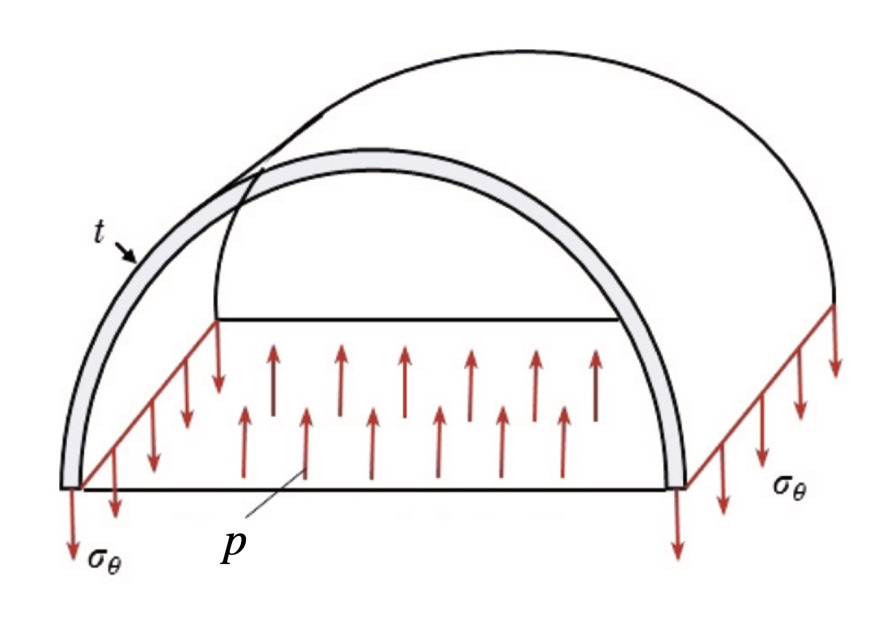
Fig. 11.3 Thin cylindrical shell under internal pressure \(p\), illustrating distribution of hoop stress \(\sigma_\theta\).#
The vertical force due to the internal pressure on a small piece of half a cylinder having length \(dz\) (see Fig. 11.2 and Fig. 11.3) is
Vertical equilibrium of the small piece of cylinder leads to: \( 2 \sigma_{\theta} t dz = 2p R_\text{i} dz\) and therefore the hoop stress is given by
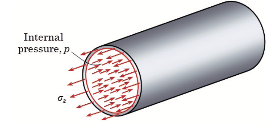
Fig. 11.4 Thin cylindrical vessel under internal pressure \(p\), showing axial stress \(\sigma_z\) acting on the end caps.#
The axial stress \(\sigma_z\) depends on the boundary conditions for the problem. If the cylinder has closed ends (see Fig. 11.4) then axial equilibrium of half a cylinder gives:
and the axial stress becomes
with \( R_\text{m} =(R_\text{o}+R_\text{i})/2\). Since \(R_\text{m} \approx R_\text{i}\):
For a cylinder having open ends (see Fig. 11.5) the pressure doesn’t act in axial direction and \(\sigma_z = 0\).
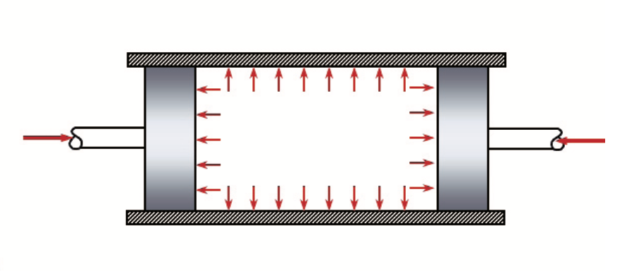
Fig. 11.5 Free-body diagram of a pressurized cylinder with end closures, illustrating the balance of internal pressure and axial forces.#
For the radial stress \(\sigma_r\) we have \(-p\leq \sigma_r \leq 0\) and because \( |\sigma_r | \ll | \sigma_z| \) and \(|\sigma_r|\ll|\sigma_{\theta}|\), the radial stress \(\sigma_r\) can be neglected.
End plates analysis
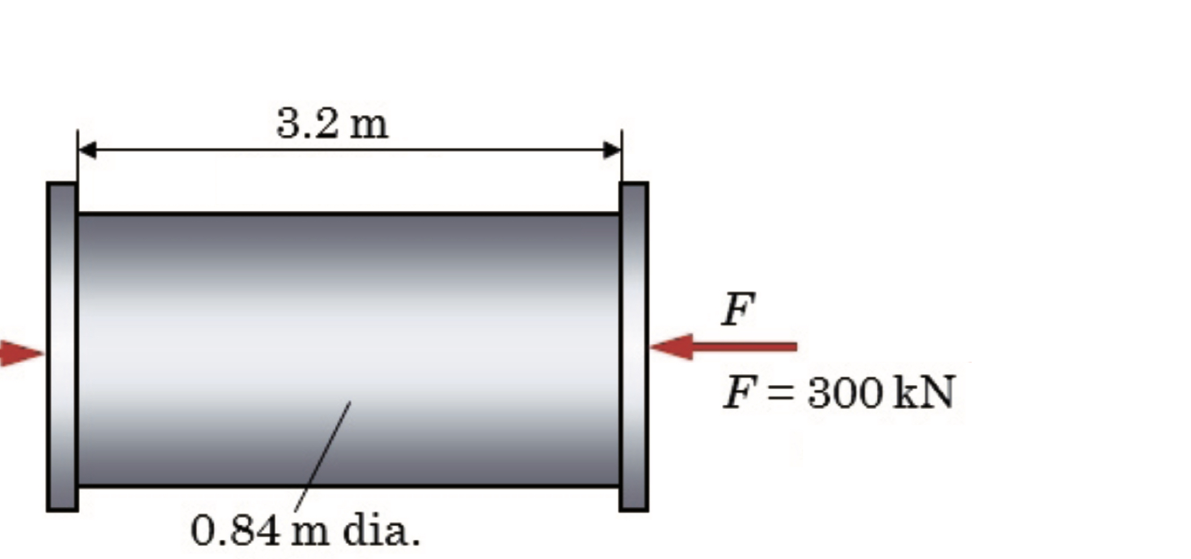
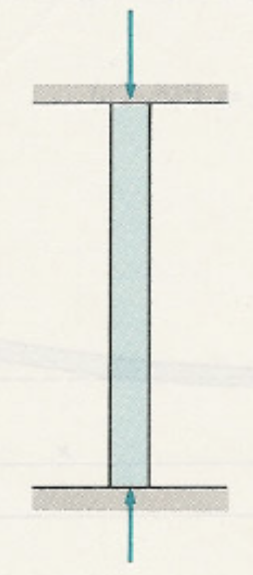
Fig. 11.6 Cylindrical bar of diameter \(0.84 , \text{m}\) and length \(3.2 , \text{m}\) subjected to axial compressive forces \(F = 300 , \text{kN}\) applied at both ends.#
For this problem the goal is to calculate the hoop and axial stresses away from the end plates of Fig. 11.6. For the cylindircal bar we have the given values \(t = 4.5 \ \rm mm\), \(p = 1.2 \ \rm MPa\) and \(F = 300 \ \rm kN\).
Solution
First we can find \(\sigma_{\theta}\) by
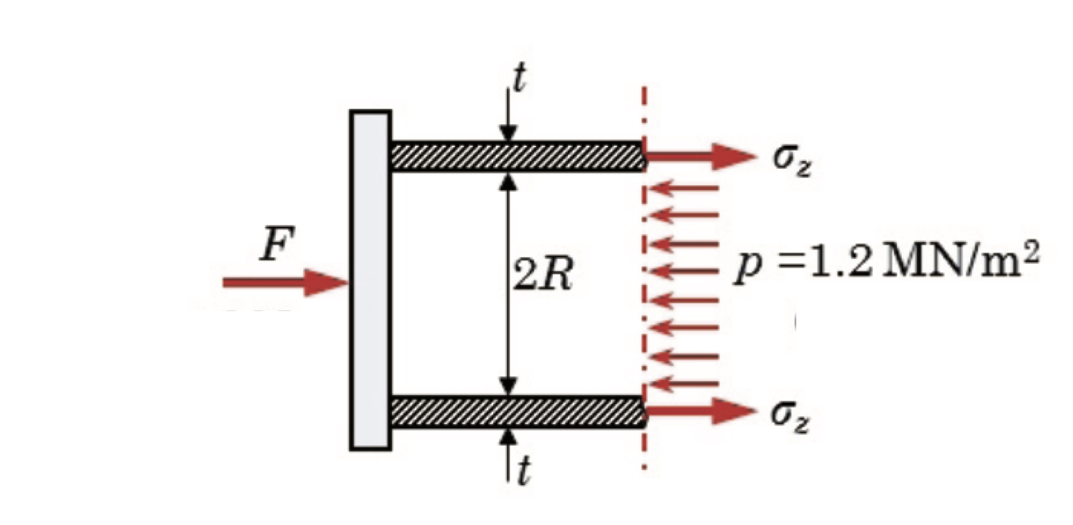
Fig. 11.7 Free-body diagram of the cylindrical vessel wall under internal pressure \(p = 1.2 ,\text{MN/m}^2\), showing the balance between the applied force \(F\) and the resulting axial stress \(\sigma_z\) acting over the wall thickness \(t\) and diameter \(2R\).#
By making a free-body diagram as in Fig. 11.7 and setting up a force balance fot \(F_H\) we gat that
Where thus \(\sigma_z\) can be found through
11.3. Pressurised thin-walled sphere#
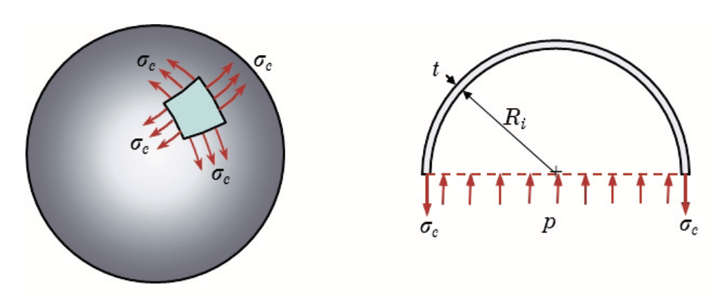
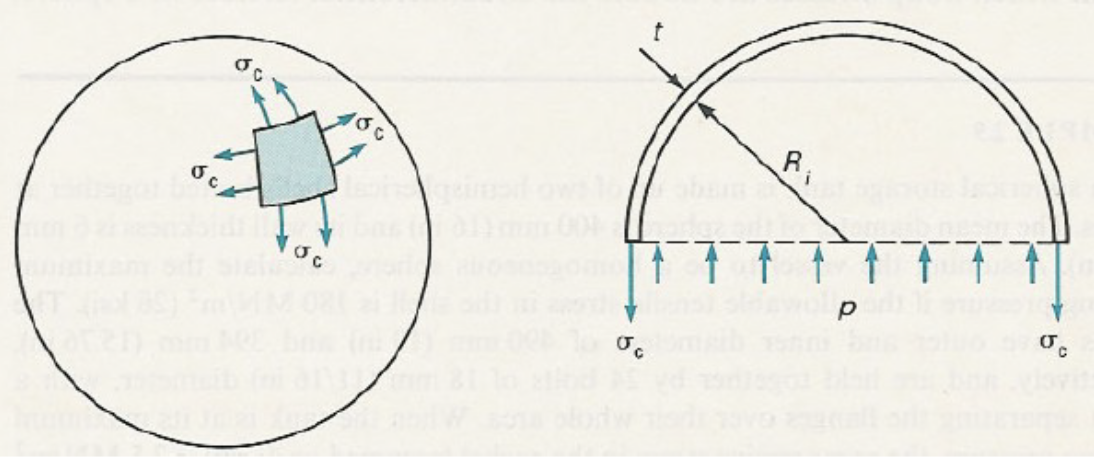
Fig. 11.8 On the left a thin spherical shell under internal pressure, showing uniform membrane (hoop) stress \(\sigma_c\) acting in all directions on the surface element is visible. On the right a free-body diagram of a hemispherical shell of radius \(R_i\) and thickness \(t\), with internal pressure \(p\) balanced by circumferential stress \(\sigma_c\) is given.#
Consider a thin-walled sphere having internal radius \(R_\text{i}\) and thickness \(t\), where \(t \ll R_\text{i}\). The sphere is internally pressurised with a pressure \(p\). Now, make a horizontal cut through the center of sphere and consider the upper half (see Fig. 11.8). Introducing the membrane stress \(\sigma_\text{c}\) and applying vertical equilibrium of the upper half of the sphere, we get:
The membrane stress \(\sigma_\text{c}\) is therefore given by
Sections 2.2.3 and 2.3 can be skipped. These are not part of the exam.
11.4. Buckling of struts and columns#
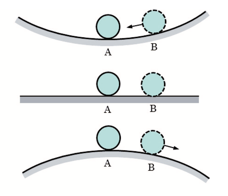
Fig. 11.9 Illustration of stability of equilibrium using a sphere on a surface. On the top we have a stable equilibrium. a small perturbation moves the sphere back to position \(A\). For the middle a neutral equilibrium. The sphere at \(B\) remains in the new position after perturbation. For the bototm an unstable equilibrium is visible. A small perturbation moves the sphere further away from position \(B\).#
Deformable structures can become mechanically unstable (buckle) if the load exceeds a certain critical load. A structure is unstable if after applying a small perturbation it will not return to its original position. Depending on the load, the structure can be stable, neutral or unstable. In Fig. 11.9 this is illustrated for a sphere on a surface in a gravity field. At the critical load a structure can go along an equilibrium deformation path different from the expected one based on the load, like an axially load beam or cylinder that moves sideways. The sideway motion is usually large and can easily lead to plastic deformation and failure of the structure. Mechanical instability (buckling) can only be predicted if geometrical nonlinearity is assumed (see Lecture 5 for an explanation of geometrical nonlinearity).
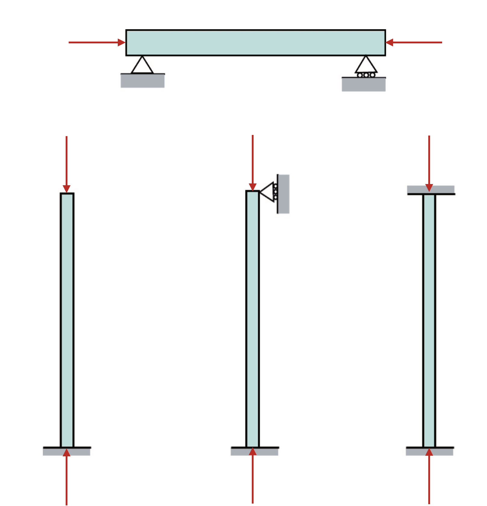
Fig. 11.10 On the top figure a strut under axial compression is shown, horizontally and supported at both ends, with forces applied along its axis. On the botom there are three vertical columns under axial compressive load, illustrating different end conditions. For the left one both ends pinned (hinged), free to rotate. The middle one has one end fixed and the other pinned, providing partial restraint. The right one has both ends fixed, preventing rotation at the supports.#
Here, we only study axially loaded beams: struts (long, slender and freely rotating at the ends) and columns (one or more fixed ends). The disicntion between these two is shown in Fig. 11.10 above. The critical buckling load \(P_\text{c}\) is given by the Euler buckling formula:
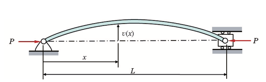
Fig. 11.11 Pinned–pinned column of length \(L\) under axial compressive load \(P\), showing lateral deflection \(v(x)\) as a function of position \(x\) along the axis, illustrating elastic buckling behavior.#
where the equivalent length \(L_\text{e}\) is defined as \(L_\text{e} = L\) for a strut (see Fig. 11.11), \(L_\text{e} = 2L\) for a column with one end fixed and the other one free (Figure 8.20), \(L_\text{e} = 0{,}5L\) for a column with both ends fixed (Figure 8.22) and \(L_\text{e} = 0{,}699L \approx 0{,}7L\) for a column with one end fixed and the other end pinned (Figure 8.23).
The expression for the critical load can also be written as an expression for the critical stress \(\sigma_\text{c}\):
where \(r=\sqrt{I/A}\) is the radius of gyration (see Appendix B.2). The ratio \(L_\text{e} / r\) is called the slenderness ratio of the strut or column. In Section 8.3.5 it is described how struts and columns having a small slenderness ratio fail by yielding, whereas struts and columns having a large slenderness ratio fail by buckling (see Fig. 11.12). The transition between these mechanisms is gradual in practise, as illustrated in Fig. 11.13.
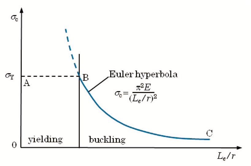
Fig. 11.12 Euler column curve showing the critical stress \(\sigma_c\) versus slenderness ratio \(L_e/r\). For short columns (region A), failure occurs by yielding at \(\sigma_Y\). For slender columns (region C), failure occurs by elastic buckling following Euler’s hyperbola \(\sigma_c = \tfrac{\pi^2 E}{(L_e/r)^2}\). The transition point \(B\) marks the boundary between yielding- and buckling-dominated behavior.#
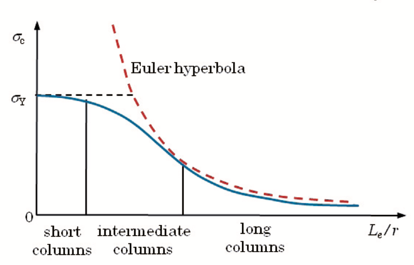
Fig. 11.13 Critical stress \(\sigma_c\) versus slenderness ratio \(L_e/r\), showing three regimes: short columns failing by yielding at \(\sigma_Y\), long columns failing by elastic buckling along Euler’s hyperbola, and intermediate columns transitioning between the two with actual strength below both limits.#
Important
For the critical buckling force for struts and columns the general relation is given by
The dependence on \(L_e\) makes it such that the three columns depicted in Fig. 11.10 get differenct critical buckling forces. For the column on the left one end is pinned (rotationally free, no translation), and the other end is free. The buckled shape is very flexible: it is equivalent to a pinned–pinned column of length \(2L\). Hence, \(\displaystyle L_e = 2L\) and the critical load is smallest. Thus we get \(\displaystyle P_c = \frac{\pi^2 EI}{4L^2}\).
For the middle column one end is fixed (no translation, no rotation), the other pinned (rotation free, no translation). The buckled shape falls between the cantilever and fixed–fixed cases. \(\displaystyle L_e \approx 0.699L \ (\approx 0.7L)\), so the critical load is larger than the pinned–pinned case but smaller than fixed–fixed. Here we get that \(\displaystyle P_c = 20.19\frac{EI}{L^2}\).
For the right column both ends are fixed, so neither translation nor rotation is allowed at the supports. This gives the stiffest condition: the buckling half-wavelength is only half the column length. Hence, \(\displaystyle L_e = \tfrac{1}{2}L\), giving the largest critical load. This gives a corresponding buckling force of \(\displaystyle P_c = \frac{4\pi^2 EI}{L^2}\).
The Sections 8.2.2–8.2.4, 8.3.2–8.3.4 and the paragraph on the secant formula (last paragraph of just before Example 8.7) are not part of the exam.
11.5. Additional Video#
This video by The Efficient Engineer provides a comprehensive visual introduction to the phenomenon of structural buckling. It begins by explaining buckling as a failure of stability under compression, and then derives the famous Euler’s formula for the critical buckling load. The video clearly breaks down the key parameters, including the importance of a column’s end conditions (effective length), its slenderness ratio, and the difference between elastic buckling and plastic failure. It also touches on more advanced topics like eccentric loading (the Secant formula) and other buckling modes like torsional and flexural-torsional buckling. This video is non mandatory and is purely to give a different perspective on the topic.
This video regarding a compressing soda can may be beneficiary to watch a well to see how a column actually buckles, or how a vessel deforms under internal pressure