

4. Beam structures#
4.1. Background: Beam bending and beam element#
In the previous chapter, truss structures were modelled and analysed. A truss structure is made up of tensile bars that are connected in their nodes to each other and/or to the fixed world. The connection point can be seen as a hinge. A truss element can only transfer an axial force \(F\) that is related to the extension ∆l of the element: \(F= \frac{E A_0}{l0}\Delta l\), where \(E\) is the elastic modulus of the material, \(A_0\) the undeformed cross-sectional area and \(l_0\) the undeformed length of the truss element.
A beam is a construction element that, just like a truss element, offers resistance to axial deformation, but also to bending and torsion. The resistance to bending results in a bending moment and the resistance to torsion in a torque.
Structures that are built from beams can be modelled and analysed with the finite element method, using beam elements. We limit ourselves here to two-dimensional beam constructions, which can be modelled with beam elements that can only deform in one plane – here the \(xy\) plane –.
4.1.1. beam bending#
The figure below shows a beam that is successively loaded by an axial force \(F\) , a shear force \(D\) and a bending moment \(M\). The horizontal and vertical displacements are represented by \(u\) and \(v\) on the right end of the beam and by the rotation \(\phi\) of the beam axis at that point.
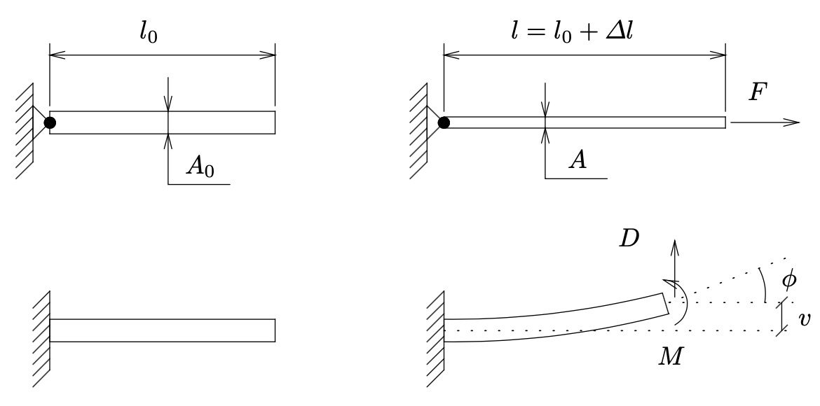
Fig. 4.8 Construction crane truss structure.#
The beam behaves itself exactly the same as a truss element with regard to the axial deformation. The extension \(Delta l= u\) is related to the axial force \(F\) via the elasticity modulus \(E\) of the material and the undistorted geometry, \(A_0\) and \(l_0\):
The vertical displacement \(v\) perpendicular to the beam axis and the rotation \(\phi\) of the beam axis are related to the shear force \(D\) and the moment \(M\):
Here we again recognize the modulus of elasticity \(E\) and the undistorted beam length \(l_0\). The distortion also appears to be dependent, and inversely proportional to, a quantity \(I\), the so-called second moment of area of the cross-section. The value of \(I\) is completely determined by the shape of the cross section. The Fig. 4.9 below illustrates that this shape is of great importance for the resistance to bending.
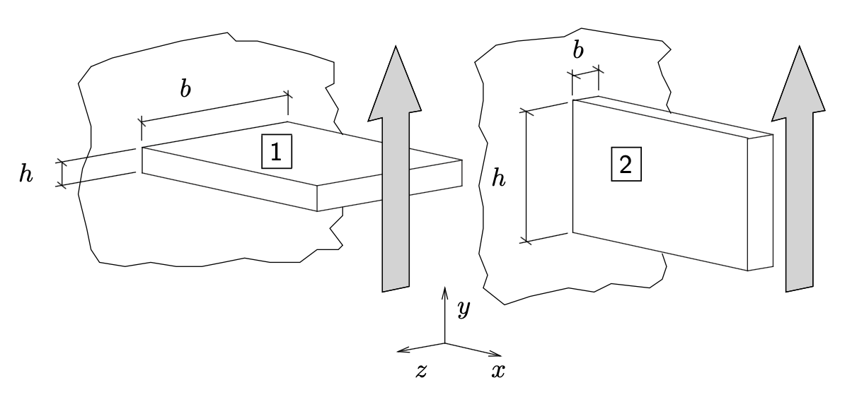
Fig. 4.9 Illustration on the importance of shape.#
With equal loading (\(D\) and/or \(M\)) beam 1 will bend more than beam 2. Without derivation – see the lecture notes of the course Mechanics (4RA00) – we state that the drawn rectangularly shaped cross section \(I\) is given by:
For beam 2, \(I\) is (much) greater than for beam 1. All kinds of cross sections can appear. Frequently the \(I\)- and box-profile are found.
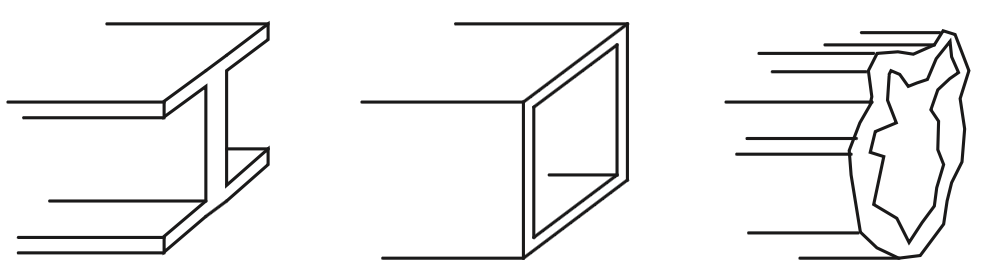
Fig. 4.10 Frequent cross section shapes.#
4.1.2. element stiffness matrix#
The mechanical behaviour of a beam element is described by a number of equations that relate the node movements and rotations to the node forces and moments. These internal node forces/moments represent the resistance to deformation. For the modelling using Mentat/MARC we use a three-dimensional beam element. This element has the MARC name elastic beam (element no. 52) and is drawn in the figure below with all 12 displacement components and rotations (the so-called degrees of freedom) and associated internal forces/moments.
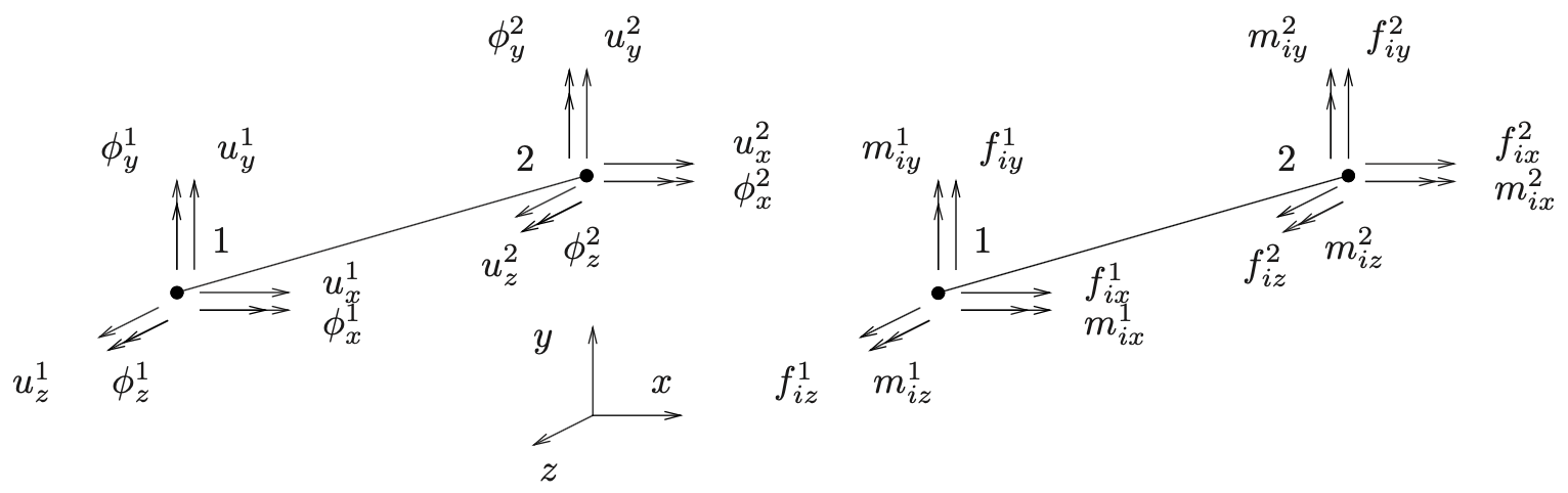
Fig. 4.11 Schematic of the three-dimensional elastic beam element (MARC element no.,52), showing at each node (1 and 2) the six kinematic degrees of freedom—translations \(u_x, u_y, u_z\) and rotations \(\phi_x, \phi_y, \phi_z\)—and the corresponding internal nodal forces \((f_x, f_y, f_z)\) and moments \((m_x, m_y, m_z)\) that resist deformation.#
Because in the context of this manual we will always use the element in the xy-plane, we must suppress some of these degrees of freedom when modelling, namely the movement in z-direction and the rotations around the x- and y-axis. The relevant degrees of freedom and the corresponding internal forces/moments are indicated in the figure below.
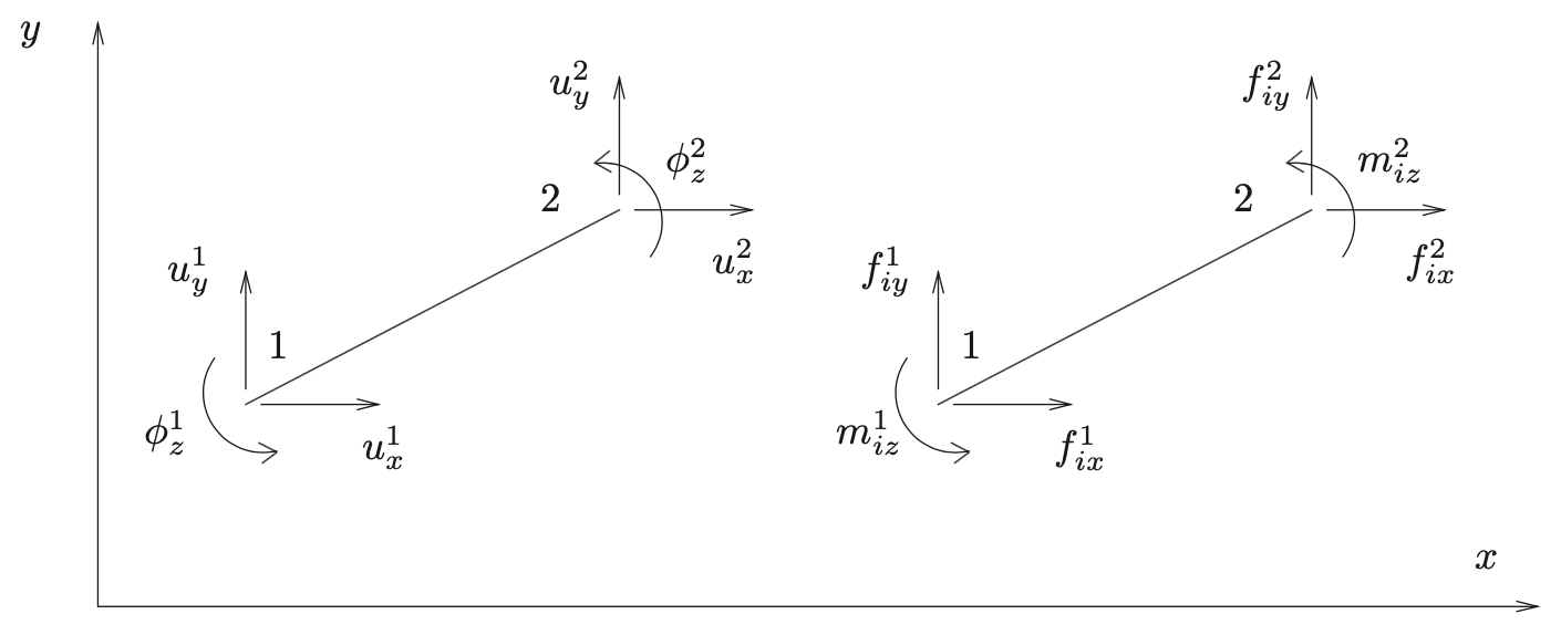
Fig. 4.12 Schematic of the two‐dimensional elastic beam element, showing at each node (1 and 2) the planar kinematic degrees of freedom—translations \(u_x\), \(u_y\) and out‐of‐plane rotation \(\phi_z\)—and the corresponding internal nodal forces \((f_{ix}, f_{iy})\) and bending moment \(m_{iz}\) that resist deformation.#
The six degrees of freedom and six force quantities are stored in columns:
The superscript \(^e\) denotes the element and \(^T\) indicates that the column is transposed. The relation between \(\col{u}^e\) and \(\coli{f}^e\) is mathematically written by using a \(6 \times 6\) matrix: the element stiffness matrix \(\mat{K}^e: \; \coli{f}^e = \mat{K}^e \col{u}^{e~i}\). In the Appendix Section 5 the stiffness matrix is explained in more detail.
4.1.3. assembly#
In the beam structure, beam elements are connected to each other. When connecting or assembling the beam elements the same considerations apply that were previously described for the truss structures: in a node, internal forces/moments of the joining elements are added together and their degrees of freedom must have equal values. When beams are interconnected, the rotations must be equal in a node in addition to the displacement components. This means that beams are not connected with hinges but are as it were welded together.
4.1.4. Boundary conditions and solving#
After prescribed displacements/rotations and/or forces/moments are applied, the unknown nodal degrees of freedom can be determined by solving a system of algebraic equations as previously explained for the truss structures. Once again, a solution can only be determined if the rigid movement of the structure is suppressed.
4.2. Two-dimensional beam structure#
In this example we consider a simple two-dimensional beam structure, as shown in the figure below. The dimensions are indicated in the figure and are in meters [m].
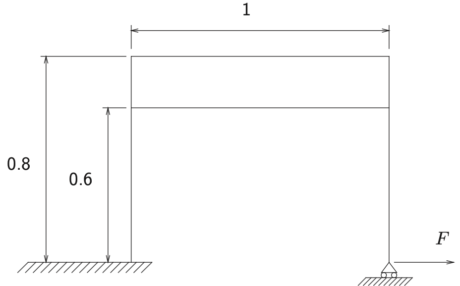
Fig. 4.13 Two-dimensional beam structure.#
All beams are undeformed and located in the \(xy\)-plane. The load \(F=1000\) [N], acts in \(x\)-direction. The beams are made of steel and the material properties are given below:
The cross sections of the beams are a square and have a surface area of \(A_0 = 0.0004\) [\(\textrm{m}^2\)].
4.2.1. Modelling and analysis#
GEOMETRY \(\&\) MESH
info
We start in the main menu. First, the geometry of the model must be defined. This is done within the GEOMETRY \(\&\) MESH submenu. First we ensure that we get a em grid on the screen with standard dimensions: \(-1 \le x \le 1 \quad\text{and}\quad -1 \le y \le 1.\). The standard spacing is 0.1 in both directions. We then immediately define line elements between relevant points in the xy plane. Nodes can be ”laid down” in grid points by clicking with the left mouse button.
GEOMETRY \(\&\) MESH
☑ GRID (Coordinate System)
(ELEMENTS) 
(ELEMENTS) ADD
Defend the line elements between the various vertices of the construction.
info
The defined elements are now subdivided into elements with a length of 0.1 [m]. The direction along the beam axis is indicated by U. The direction perpendicular to the beam axis is indicated by V.
SUBDIVIDE (Operations)
DIVISIONS
Enter number of divisions in the U, V and W: 6, 1, 1
ELEMENTS
Enter subdivide element list:
Now select the desired elements.
The other elements must also be divided in an analogous way.
info
We do not need the grid any more. Switch it off and select  .
info
To reduce coincidental nodes to a single point, the SWEEP button is selected followed by a number of other actions that speak for themselves.
SWEEP (Operations)
(SWEEP) ALL
(REMOVE UNUSED) NODES
(REMOVE UNUSED) POINTS
info
We will now enter the geometric parameters of the cross section. First we have to specify the element type by turning off (TRANSVERSE SHEAR) , whereby the element type 52 is selected.
Next, we specify the properties of the cross section: the surface and the second moment of area. We then specify in relation to which axes these are defined.
GEOMETRIC PROPERTIES
NEW (STRUCTURAL)
3-D
SOLID SECTION BEAM
PROPERTIES
ELEMENT TYPES
(TRANSVERSE SHEAR) ☑ → ☐
OK
(PROPERTIES)
ENTERED
info
By selecting ENTERED (values) the menu is adjusted so that we can enter data.
With the given \(A_0 = 0.0004\) [m] we know that \(b = h = 0.02\) [m] and therefore \(I_{xx} = I_{yy} = \frac{1}{12}(0.02)^4 \; [\textrm{m}^4]\).
Area: 0.0004
\(I_{xx}\): (0.002^4)/12
\(I_{yy}\): (0.002^4)/12
info
What are \(I_{xx}\) and \(I_{yy}\)? Well, it has been described in the foregoing that we use a three-dimensional beam element for modelling. Although we only use this element in the xy plane, it is suitable for modelling three-dimensional beam constructions. In that case, bending around two axes can occur and two second moments of area will play a role. To be able to quantify and enter it into the program, we must define a local coordinate system for each beam element. \(I_{xx}\) and \(I_{yy}\) are the second moments of area relative to the local \(x\) and the local \(y\) axes respectively.
The \(z\) axis of the local element coordinate system always lies along the element axis and is positively oriented from node 1 to node 2. The user (you) must define the local \(x\) axis. To that end, we must specify the global coordinates of a spatial point. The connecting line between this point and the first element node defines a flat plane together with the beam axis. In that plane the local \(x\) axis is perpendicular to the beam axis. The local \(y\) axis is now also fixed: starting at the first element node and perpendicular to the plane of the local \(x\) and the local \(z\) axes such that the \(xyz\) system is according to the corkscrew rule.
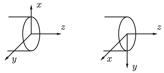
Fig. 4.14 corkscrew rule#
All this seems complicated and it is, at least when three-dimensional beam structures must be modelled. Because we limit ourselves to two-dimensional constructions in the \(x\) plane, we have it a lot easier. To define the local \(x\)-axis, select a point at the global z-axis – so this is a point on a line perpendicular to the \(xy\) plane (screen) – for example, [0 0 1].
(VECTOR DEFINING LOCAL ZX-PLANE)
COMPONENTS IN GLOBAL SYSTEM
VECTOR
Enter first component: 0
Enter second component: 0
Enter first third: 1
OK
(ELEMENTS) ADD
Enter geometry add element list:  (All existing)
info
Now we are going to define the material properties of the elements. To do this, we select MATERIAL PROPERTIES and specify the values of the Young’s modulus and the Poisson’s ratio.
MATERIAL PROPERTIES
NEW
STANDARD
STRUCTURAL
Young’s modulus: 2.1e11
Poisson’s ratio: 0.3
OK
(ELEMENTS) ADD
Enter add material element list: (All existing)
info
Finally, we apply the boundary conditions. The naming of the six degrees of freedom at the node of the three-dimensional beam element is as follows:
First, we suppress the \(z\)-displacement and the rotation around \(x\)- and \(y\)-axes in all nodes.
BOUNDARY CONDITIONS
NEW (STRUCTURAL)
FIXED DISPLACEMENTS
PROPERTIES
; ☑ Displacement Z
☑ Rotation X
☑ Rotation Y
OK
(NODES) ADD
Enter add apply node list: (All existing)
Enter the desired boundary conditions and nodal force (see figure).
info
To make all defined boundary conditions visible select ☑ identify in the tab BOUNDARY CONDITIONS
info
We are back in the main menu and have now finished all the buttons. The model of the construction is almost ready. However, a few essential items are still missing and we must specify these in the JOBS tab.
JOBS
NEW
STRUCTURAL
info
The load acting on the structure can be composed of the defined boundary conditions in PROPERTIES → INITIAL LOADS Always check if the desired load has been applied.
info
The desired calculation results, to be viewed afterwards, must be selected in PROPERTIES → JOB RESULTS from a large number of options. We choose:
PROPERTIES
(ANALYSIS DIMENSION)
3-D
JOB RESULTS
(AVAILABLE ELEMENT SCALARS)
☑ Beam Axial Force
☑ Beam Bending Moment Local X
☑ 1st Comp of Total Strain
☑ 2nd Comp of Total Strain
Comp of Total Strain
OK
OK
info
At an earlier stage we opted for line elements. However, the MARC calculation program has a number of line element types. We choose element no. 52 here.
ELEMENT TYPES (Element Types)
(ANALYSIS DIMENSION)
3-D
TRUSS/BEAM
(THIN ELASTIC BEAM) 52
OK
Enter element list: (All existing)
info
The model is now ready. We now need to save the model, so that we can adjust it later, if necessary.
| file | → | save as | → | File name: beam1 | → | SAVE |
info
The model of the construction can now be analysed. This is done with the finite element method program MARC. This calculation program can be started from Mentat. For this we go to JOBS.
JOBS
RUN
SUBMIT (1)
info
The MARC calculation program is now started and the model calculated. The (RUN)-menu provides information about the progress of the calculation. The word ”working” appears in the status menu. When MARC gives the status ”ready”, the calculation is finished. If everything went well, the (RUN)-menu will display exit number 3004. The results of the calculation can now be viewed with Mentat.
4.2.2. Results#
Let’s assume everything went well and we can see the results.
info
We select in the main menu RESULTS. The results of the calculation by MARC have been written in the file with extension .t16 (or .t19), which is read by Mentat after it has been opened.
RESULTS
file → open default
(Fill view)
(DEFORMED SHAPE)
DEFORMED & ORIGINAL
(DEFORMED SHAPE) SETTINGS
(DEFORMED SCALING) ● Automatic
info
The Beam Axial Force and the Beam Bending Moment Local X around the local \(x\)-axis in the beam element can be visualized with different colour coding.
MODEL PLOT
(SCALAR PLOT) SCALAR
● Beam Axial Force
(SCALAR PLOT)
BEAM CONTOURS
info
The colours do not indicate the precise numerical value of these quantities, because certain averaging procedures have been applied. The exact value of the axial force in a beam element can be read as follows.
(SCALAR PLOT)
NUMERICS
ISOLATE
(ISOLATE ELEMEND) ADD
select element  (End list)
info
The value of the force can now be read at the two nodes between which the element is located. With positive force being a tensile force, with negative value a compressive force. Multiple elements may be selected simultaneously. However, the specified elements must not be adjacent to each other, because then again average node values appear.
info
When we have studied the results sufficiently, it is possible that we will come to
the conclusion that the model needs to be adjusted. The file beam1_job1.t16
must first be closed, after which the model file beam1.mud can be opened and
modified. To remove the colour bar that is still present, you can select in the menu (SCALAR PLOT) → → OFF.
| file | → | close |
info
The model file (beam1.mud) is reopened immediately upon closing the *.t16 file. If this does not happen, it can still be opened via file in the main navigation menu. If we have had enough, we can stop Mentat.
| file | → | exit |
4.3. Exercises#
A few simple beam structures are presented in this section, that can be modelled and analysed with Mentat/MARC. Use the three-dimensional beam element in all cases (element no. 52) and suppress the deformations from the \(xy\)-plane.
4.3.1. Simple beam bending#
In the Fig. 4.15 below a clamped beam is drawn, of which the relevant dimensions and (linearly elastic) material parameters are given.
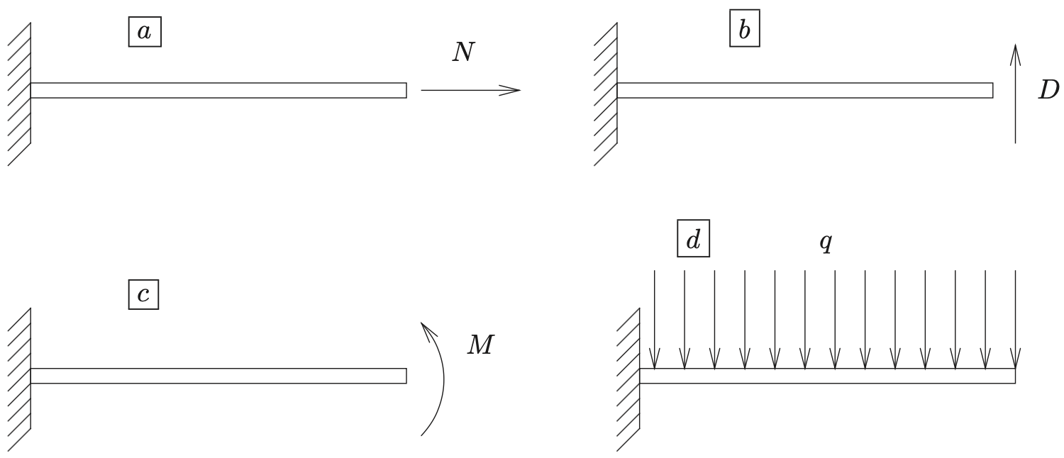
Fig. 4.15 Simple beam bending structure.#
Property |
Symbol |
Value |
Units |
|---|---|---|---|
Length |
\(l_0\) |
2 |
m |
Height |
\(h\) |
0.1 |
m |
Width |
\(b\) |
0.1 |
m |
Young’s modulus |
\(E\) |
\(2\!\cdot\!10^{11}\) |
N m\(^{-2}\) |
Poisson’s ratio |
\(\nu\) |
0.3 |
– |
Density |
\(\rho\) |
7850 |
kg m\(^{-2}\) |
Exact solutions for horizontal movement \(u\), vertical displacement \(v\) and rotation \(\phi\) from the end of the beam are given in the table below for the different loading conditions. In these relationships \(A_0\) is the undistorted cross-sectional area (\(A_0 = bh\)) and \(I\) the second moment of area (\(I= \frac{1}{12} bh^3\)). The load consists of either a force \(N\) or \(D\) [N] or a bending moment \(M\) [Nm] or a distributed load \(q\) [N/m] resulting from its own weight.
Case |
\(u\) |
\(v\) |
\(\phi\) |
|---|---|---|---|
a |
\(\dfrac{N\,l_0}{E\,A_0}\) |
0 |
0 |
b |
0 |
\(\dfrac{D\,l_0^{3}}{3\,E\,I}\) |
\(\dfrac{D\,l_0^{2}}{2\,E\,I}\) |
c |
0 |
\(\dfrac{M\,l_0^{2}}{2\,E\,I}\) |
\(\dfrac{M\,l_0}{E\,I}\) |
d |
0 |
\(\dfrac{q\,l_0^{4}}{8\,E\,I}\) |
\(\dfrac{q\,l_0^{3}}{6\,E\,I}\) |
Calculate the deformation of the beam for each of the above load situations and compare the result with the exact solution according to the formulas in the table. Use 40 elements.
The solution, calculated with the finite element method, is an approximation of the exact solution, so that in some cases the deviation can be considerable. What could be the cause of the difference in results, in particular for the loading condition in d? How could this difference be reduced?
4.3.2. Beam structure I#
A construction is drawn in the left-hand side of the figure below.
It consists of two beams that are attached to the fixed world with a clamp.
The structure is loaded with a vertical force \(F = 8000\;\text{N}\).
The undeformed length of both beams is \(l_{0} = 1\;\text{m}\).
The beams have a square cross-section with an area \(A_{0} = 0.01\;\text{m}^2\).
The material behaviour is linear-elastic with a modulus of elasticity
\(E = 10^{11}\;\text{N/m}^2\) and Poisson’s ratio \(\nu = 0.3\).
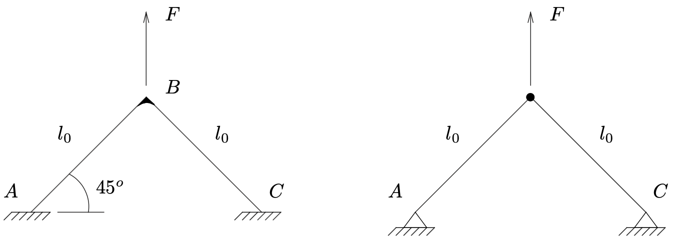
Fig. 4.16 Schematic of a V-shaped two-beam frame (each beam of undeformed length \(l_0\)) clamped at supports \(A\) and \(C\) and loaded at the apex \(B\) by a vertical force \(F\).#
4.3.2.1. Tasks#
Beam-element model
Model the construction with 40 beam elements and calculate the displacement of the point where the load is applied.\[v = 7.921 \times 10^{-6}\;\text{m}\]Question: Is it necessary to model both beams?
Truss-element model
Model the same construction but now with truss elements and compare the result.\[v = 8 \times 10^{-6}\;\text{m}\]Vary the boundary conditions and the cross-sectional area of the beam/truss elements.
Longer beams
Model the construction anew but now with beam lengths of \(l_{0}=2\;\text{m}\).
Again use 40 elements and compare the difference between beam and truss elements.\[v_{\text{beam}} = 15.960 \times 10^{-6}\;\text{m},\qquad v_{\text{truss}} = 16.000 \times 10^{-6}\;\text{m}\]
4.3.3. Beam structure II#
In Fig. 4.17 below a beam construction is drawn that consists of three beams with lengths \(l_{0}=1\;\text{m}\), a square cross-section with area \(A_{0}=0.0004\;\text{m}^{2}\), an elastic modulus of \(E = 2\!\cdot\!10^{11}\;\text{N/m}^{2}\) and a Poisson’s ratio of \(\nu = 0.3\).
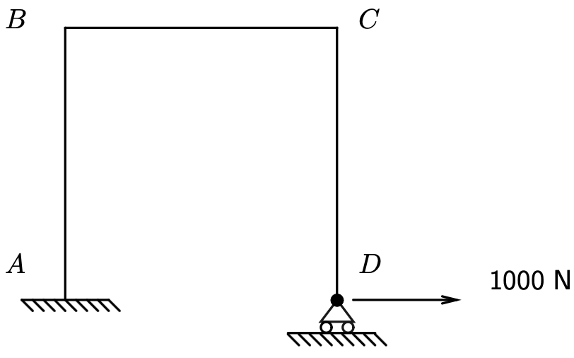
Fig. 4.17 Schematic of a three-member frame: uprights \(AB\) and \(CD\) (each length \(l_{0}\)) joined by top beam \(BC\), fixed at support \(A\) and pinned at \(D\), with a horizontal \SI{1000}{N} load applied at joint \(D\).#
4.3.3.1. Tasks#
Beam-element model
Model the structure with beam elements (beam nr. 52) and calculate the
reaction forces and moments.Stress locations and magnitudes
Determine where the largest stresses occur in the construction and compute
their magnitudes, using\[ N = \sigma_{0}\,A_{0}, \qquad M_{xx} = \frac{I}{h/2}\,\sigma_{b,\max}, \]where
\(\sigma_{0}\) is the axial stress due to the axial force \(N\), and
\(\sigma_{b,\max}\) is the maximum bending stress produced by the beam
bending moment \(M_{xx}\) about the local \(x\)-axis.
4.3.4. Beam structure III#
A beam structure shown in Fig. 4.18 below is made from a number of beams of equal length \(l_{0}=1\;\text{m}\). Relevant dimensions and boundary conditions are indicated in the sketch. Each beam has a box-profile cross-section; two options are to be analysed:
The elastic modulus is \(E = 2 \times 10^{11}\;\text{Pa}\) and Poisson’s ratio \(\nu = 0.3\).
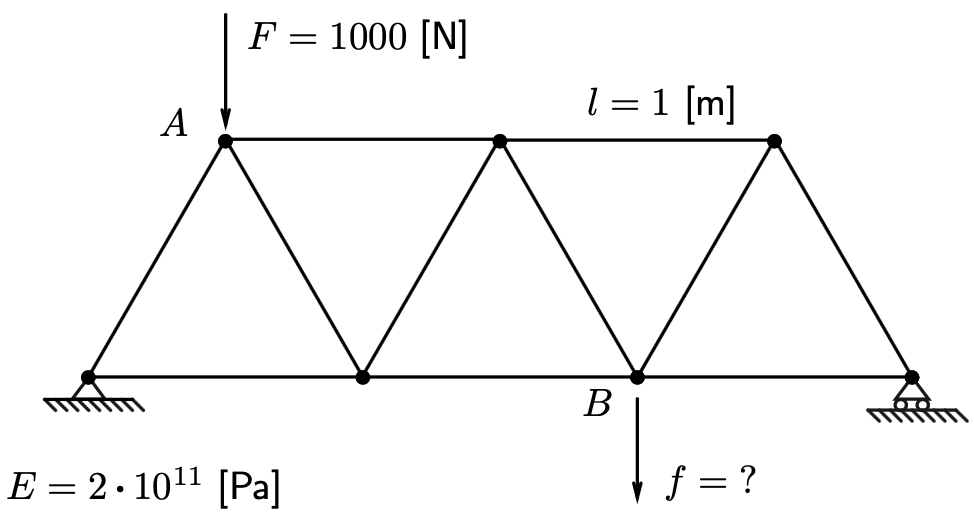
Fig. 4.18 Schematic of a truss-like beam assembly (members of length \(l_{0}\)) fixed at the left support and roller-supported at the right, loaded by a vertical \(F=1000\;\text{N}\) at joint \(A\). The unknown reaction \(f\) is to be determined at joint \(B\). Two alternative box-profile cross-sections are provided below the structure.#
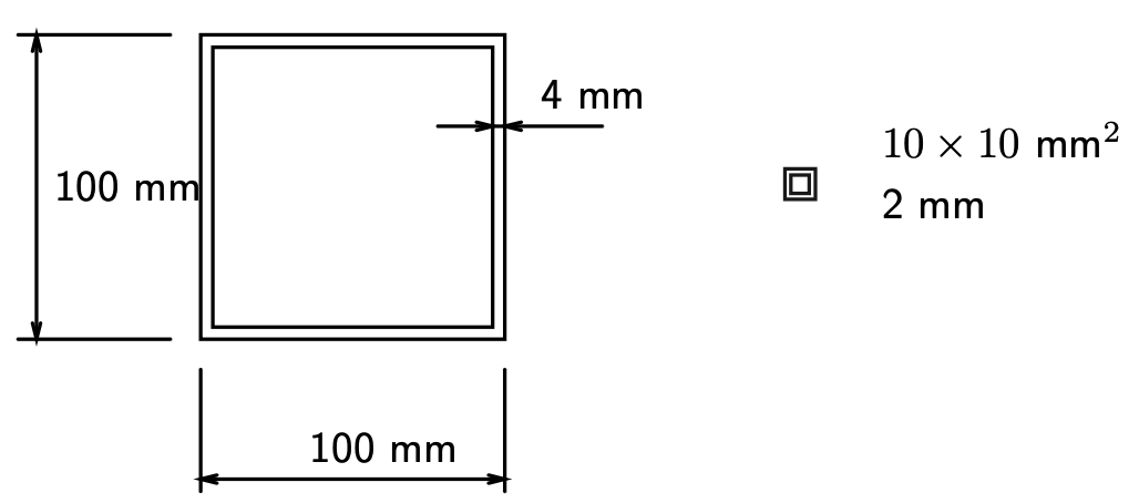
Fig. 4.19 Two alternative box-profile cross-sections provided for the structure.#
4.3.4.1. Tasks#
Beam-element model
Model the structure twice—once for each of the cross-sections above—and
compute the vertical displacement of point \(B\).Truss-element model
Model the same geometry with truss elements. Compare the displacement of
point \(B\) with the beam-element results. What can you conclude?