
3. Two-dimensional truss structure#
In this example we consider a simple two-dimensional truss, see Fig. 3.17.
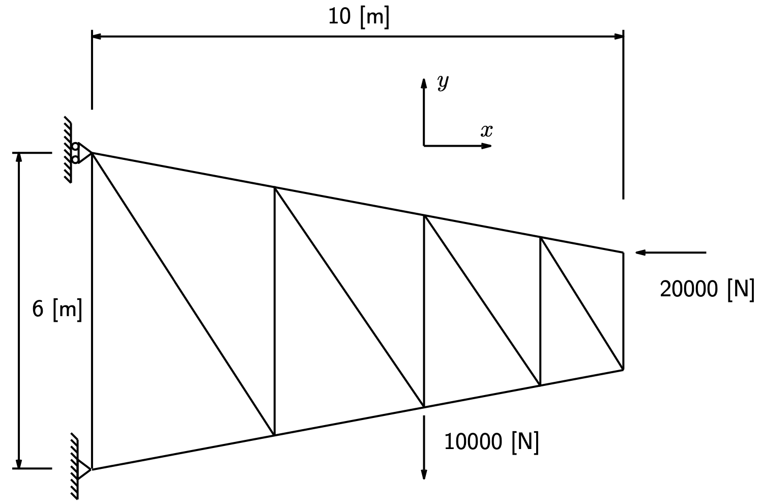
Fig. 3.17 truss example#
All truss elements are undeformed and placed in the \(xy\) plane. The same holds for the load. As a result the deformed truss will also be situated in the \(xy\) plane.
The cross section of the truss elements is depicted in Fig. 3.18.
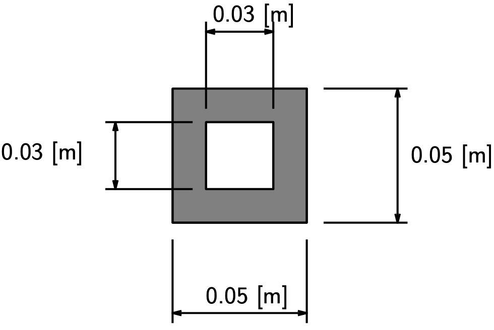
Fig. 3.18 truss cross-section#
The shape of the cross-section is irrelevant because we assume that the bars are only axially loaded. The cross-sectional area is essential for the behaviour and can be calculated with the dimensions shown in Fig. 3.18: \(A_0 = 1.6· 10^{−3} \: [\textrm{m}^2]\).
It is assumed that the bars in the framework are made of steel. The values of the stiffness parameters are then:
3.1. Modelling#
GEOMETRY \(\&\) MESH
info
We start in the main menu and gradually work from left to right. First of all, the geometry of the model must be defined. This happens within the submenu GEOMETRY \(\&\) MESH . We will first build the truss from points and straight lines. The spatial coordinates of the points must be entered via the keyboard. Some possibilities are demonstrated below.
GEOMETRY \(\&\) MESH (Basic Manipulation)
(POINTS) ADD
Enter point coordinates (\(X\)): 0
Enter point coordinates (\(Y\)): 0
Enter point coordinates (\(Z\)): 0
Point added
Enter point coordinates (\(X\)): 10, 2, 0 (or: ** 10 2 0**)
info
The last point is placed outside of the screen. Use the button fill view (Ⅱ) to make both points visible.
 (Fill view)
Enter point coordinates (\(X\)): 10, 4, 0
Enter point coordinates (\(X\)): 0, 6, 0
info
All points have now been entered. However, the numbers cannot be seen on the screen. We will ensure that this is done with the following commands. We will also ensure that numbers of curves, nodes and elements are displayed in the future. Finally, the regenerate button (Ⅱ) must be used to redraw the model.
| view | → | plot control | → | nodes | (SETTINGS) | → | ☑ labels → OK |
| → | elements | (SETTINGS) | → | ☑ labels → OK | |||
| → | points | (SETTINGS) | → | ☑ labels → OK | |||
| → | curves | (SETTINGS) | → | ☑ labels → OK | |||
| → | OK | ||||||
 (Regenerate)
info
Then the straight lines between the various points are defined. To that end we must first make it clear that these are straight lines, since there are more possibilities, but these do not matter to us now. Click on  to make the drop-down menu visible and select LINE .
(curves)
LINE
(curves) ADD
Enter line points: 1
Enter line points: 2
Curve added
Enter line points: 2, 3
Curve added
Enter line points: 3, 4
Curve added
Enter line points: 4, 1
Curve added
info
As mentioned earlier, there is a fundamental difference between points and lines with which we define the shape of our truss and nodes and elements with which we define the finite element model. We are going to do the latter now and we must first indicate that we want to use line elements.
(ELEMENTS)
LINE(2)
info
Lines which we defined earlier are now converted to line elements (CONVERT). A line can, if desired, be subdivided in more line elements. (DIVISIONS). The direction along the line is U. The direction perpendicular to the line is Ⅴ.
CONVERT (Operations)
CONVERT
CURVES
DIVISIONS
Enter the number of convert divions 4
info
How the length of the generated elements changes along the line can be defined by specifying a bias factor. This bias factor has a value between \(-1\) and \(+1\). If the value is zero (\(0\)) then the generated elements in the relevant direction will have the same length. A positive bias factor results in the elements becoming smaller in the positive direction along the line. The positive direction of the line can be shown as follows.
| view | → | plot control | → | curves | (SETTINGS) | → | ☑ direction | → | OK |
| → | OK | ||||||||
(Regenerate)
info
With a negative bias factor the elements increase in the positive direction along the line. Usually, a number of attempts have to be made before the desired element distribution is obtained. Undesired distributions can be undone via the undo button
 (Ⅱ).
BIAS FACTOR
Enter the convert bias factor in U: 0.3333
CONVERT
Enter convert curve list: 1
Enter convert curve list:  (End list)
info
With selecting it is indicated that the selection is completed. This (End list)
command can be given in three ways: entering # on the keyboard, via clicking the
button (Ⅵ) or by clicking the right-mouse button in the model window (Ⅶ).
BIAS FACTOR
Enter the convert bias factor in U: -0.3333
CONVERT
Enter convert curve list: 3 (End list)
info
Now you are going to insert the rest of the elements of the truss.
GEOMETRY \(\&\) MESH
(ELEMS)
Enter element node (1): 10
Enter element node (2): 2
Element added
Enter element node (1): 10, 1
Element added
Enter element node (1): 2, 9
Element added
Enter element node (1): 9, 3
Element added
Enter element node (1): 3, 8
Element added
Enter element node (1): 8, 4
Element added
Enter element node (1): 4, 7
Element added
Enter element node (1): 7, 5
Element added
Enter element node (1): 5, 6
Element added
info
When creating the element distribution, it is possible that two nodes coincide in a spatial point. If nothing is done about this, a ”hole” will arise during loading of the structure, in fact, the calculation cannot even be performed because of numerical problems, which will inevitably occur. To reduce coincident nodes to a single point, SWEEP is selected, followed by a number of other actions that speak for themselves.
SWEEP (Operations)
(SWEEP) ALL
(REMOVE UNUSED) NODES
(REMOVE UNUSED) POINTS
info
Although all curves have been converted into elements, we still see “orange” lines. This colour is used for elements that are ”attached” to curves. This is not important to us and can be undone, after which all elements are signed “black”.
ATTACH (Operations)
(DETACH)ELEMENTS
info
Many operations apply to all elements (curves/elements/…) within our model. To
select all elements of the requested type, there is the button  (All existing). (Ⅵ)
Enter detach element list: (All Existing)
info
Elements and nodes are now defined. GEOMETRY \(\&\) MESH has ended. Via the main navigation window, view → plot control, we can remove the checkmarks at Points and Curves to make sure they are no longer displayed; close by clicking on OK. To make the changes visible press (Regenerate).
(Regenerate)
info
Now we will specify the size of the cross-sectional area of the bar elements.
GEOMETRIC PROPERTIES
NEW (STRUCTURAL)
3-D
TRUSS
PROPERTIES
Cross Section Area: 1.6e-3
OK
(ELEMENTS) ADD
Enter geometry add element list: (All existing)
info
Now we are going to specify the material properties of the elements. In the main menu (Ⅳ) we select MATERIAL PROPERTIES and give the values of the Young’s modulus and the Poisson’s ratio.
MATERIAL PROPERTIES
NEW
STANDARD
STRUCTURAL
Young’s Modulus: 2.1e11
Poisson’s Ratio: 0.3
OK
(ELEMENTS) ADD
Enter add material element list: (All existing)
info
After determining the geometry, geometry properties and material properties, we can begin to introduce the boundary conditions. So where and how is the construc- tion fixed to the world and where and how do the various forces meet as indicated in the construction drawing.
BOUNDARY CONDITIONS
NEW (STRUCTURAL)
FIXED DISPLACEMENTS
PROPERTIES
☑ Displacement \(X\)
☑ Displacement \(Y\)
OK
(NODES) ADD
Enter add apply node list: 1, (End list)
NEW (STRUCTURAL)
FIXED DISPLACEMENTS
PROPERTIES
☑ Displacement \(X\)
OK
(NODES) ADD
Enter add apply node list: 10, (End list)
NEW (STRUCTURAL)
POINT LOAD
PROPERTIES
☑ Force \(Y\)
Enter value for ’\(y\)’: -10000
OK
(NODES) ADD
Enter add apply node list: 3, (End list)
NEW (STRUCTURAL)
POINT LOAD
PROPERTIES
☑ Force \(X\)
Enter value for ’\(x\)’: -20000
OK
(NODES) ADD
Enter add apply node list: 3, (End list)
info
The boundary conditions are prescribed. You can make them all visible by selecting ☑ identify.
info
We now finished all tabs. The model of the truss is almost ready. Some essential items are missing which you have to specify in the tab JOBS .
JOBS
NEW
STRUCTURAL
info
The truss considered by us is two-dimensional, that is to say that the construction is assumed to deform in a flat plane (the \(xy\) plane). This should be indicated in the menu PROPERTIES → ANALYSIS DIMENSION.
The load on the structure can be compiled from the defined boundary conditions in PROPERTIES → INITIAL LOADS. When boundary conditions are already selected (always check!), you obviously do not have to do anything.
The desired, retrospective, calculation results must be selected in PROPERTIES → JOB RESULTS from a large number of possibilities. We choose stress (Stress) and strain (Strain) from a list. The list can be scrolled with a slider.
PROPERTIES
(ANALYSIS DIMENSION)
2-D
INITIAL LOADS
☑ apply1, ☑ apply2, ☑ apply3, ☑ apply4
OK
JOB RESULTS
(AVAILABLE ELEMENT TENSORS)
☑ Stress
☑ Total Strain
OK
OK
info
At an earlier stage we opted for line elements. However, the calculation program MARC has a number of types of line elements. We choose element number 9 here.
ELEMENT TYPES (ELEMENT TYPES)
(ANALISYS DIMENSION)
3-D
TRUSS/BEAM
(TRUSS) 9
OK
Enter element list: (All existing)
info
The model is ready. We now have to save that model on the hard drive, so that we can adjust it later if necessary. If we make a complicated model, it is wise to save earlier, this in view of an unexpected computer failure. Please note that there can be no spaces in both the directory and the file name.
| file | → | save as | → | File name: Frame1 | → | SAVE |
3.2. Background: The system of node equations#
As previously described, a truss element can only be axially loaded, which results in a change in length. The relation between ∆l and axial force F is:
where \(l_0\) is the length of the undeformed truss element, \(A_0\) is the cross-sectional area and \(E\) the elasticity modulus of the material.
When modelling a truss, use is made of such truss elements, which are connected in their nodes with
each other or with the fixed world. After applying the boundary conditions, the deformation of the framework can be calculated. This is done by the finite elements method program MARC and in order to understand what exactly is happening, we need to know a bit more about the way in which the mechanical behaviour of a truss element is described.
3.2.1. element stiffness matrix#
The mechanical behaviour of a two-dimensional truss element is described by a number of equations. These relate the node displacements to the forces needed to realize these displacements. These forces are called internal nodal forces. They represent the resistance to deformation, in other words, the resistance of the element to the displacement of its nodes. They can thus be regarded as forces exerted by the element, i.e. from the inside out at the nodes, if they are displaced.
In the truss considered, each truss element is in the xy plane. In that case, two displacement compo- nents and two internal node force components are relevant in each node. They are indicated in Fig. 3.19 below.
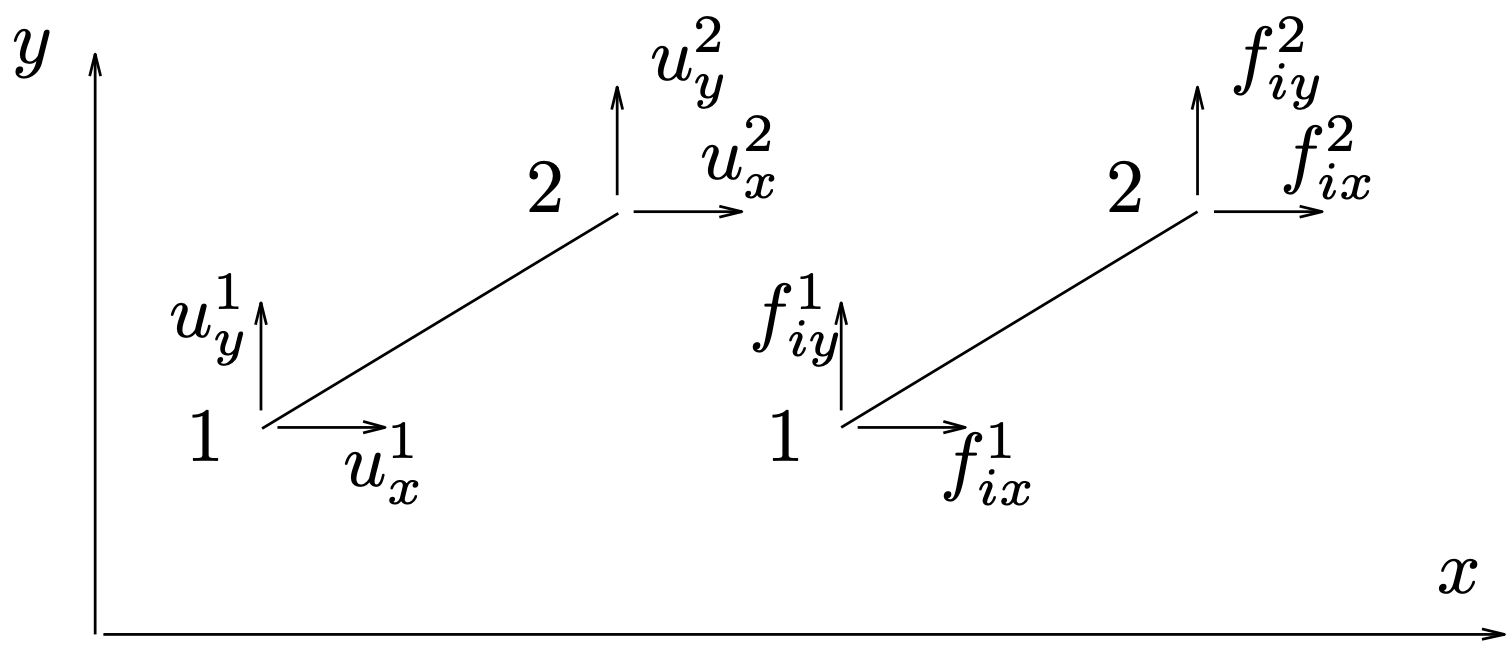
Fig. 3.19 displacement components#
The four displacement components, also called degrees of freedom, and the corresponding four force components are stored in columns:
The index \(^e\) indicates the element and index \(^T\) That the column is transposed. The relation between \(\col{{u}}^e\) and \(\coli{{f}}^{\,e}\) is mathematicall in a \(4 \times 4\) matrix: the element stiffness matrix \(K^e\).
The element stiffness matrix can be calculated for each element and depends on the geometry of the element, the material properties and the position of the element in the space, indicated by \(c = \cos{\alpha}\) and \(s = \sin{\alpha}\), where \(\alpha\) is the angle between the element axis and the \(x\) axis.
3.2.2. assembly#
A large number of elements are connected to each other in the construction. This linking of the elements in FEM terminology is called assembly. It is obvious that there is a form of “summation” of the equations, which describe the behaviour of each element separately. It comes down to the fact that in a node where multiple elements are connected, the internal node forces of all those elements are added up. In the figure below this is shown schematically for a node where three elements come together. The elements have been cut loose near the node. They are not drawn; their axial internal forces are indicated.
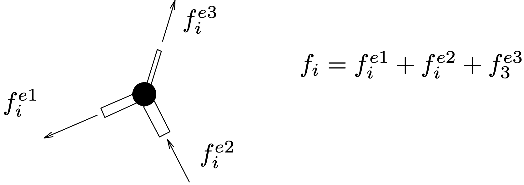
Fig. 3.20 assembly visual#
The result of assembly is a system of equations, with which the displacements of all nodes in the structure are related to the internal node forces acting on those nodes. We store the components of these displacements and forces in the columns \(\bar{\col{u}}\) and \(\bar{\coli{f}}\) so we can write this system as follows:
The matrix \(\bar{K}\) is the construction stiffness matrix. for a 2-dimensional truss with \(np\) nodes this results in a \(2np \times 2np\) matrix. From the information provided by us via Mentat, the calculation program MARC compiles the matrix \(\bar{K}\).
3.2.3. node equilibrium#
Now it is known which forces the elements exert on the nodes when they are displaced. In each node, this internal force must be in balance with the force \(f_e\), which is exerted by the environment on that node, as shown in Fig. 3.21 below.
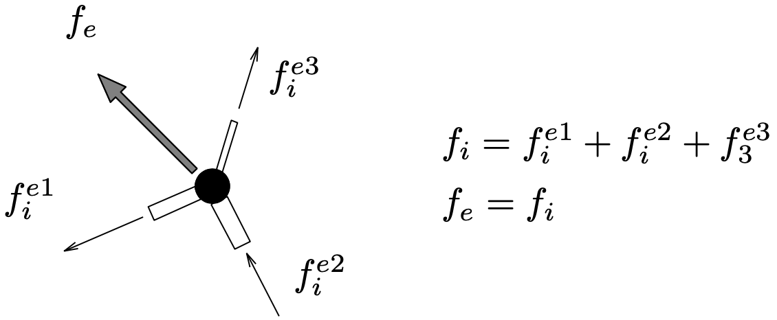
Fig. 3.21 node equilibrium#
This external nodal force is contained in the column \(\bar{\cole{f}}\) . For all nodes together, this requirement of node equilibrium means that the following system must comply with:
3.2.4. boundary conditions#
The columns \(\bar{\col{u}}\) and \(\bar{\cole{f}}\) are not completely filled with unknown quantities. After all, a number of junction displacements and node forces are known. We have prescribed them as boundary conditions. The MARC program takes these boundary conditions into account and reduces the system \(\bar{K}\,\bar{\col{u}} = \bar{\cole{f}}\) to a smaller system \(K\,\col{u} = \cole{f}\) with a fully known right member \(\cole{f}\) and a completely unknown column \(\col{u}\).
3.2.5. solution process#
The system of equations \(K\,\col{u} = \cole{f}\) is solved. Because the system is written in matrix form, implies that the inverse \(K^{−1}\) of \(K\) has to be determined:
When all nodal displacements are know, the unknown nodal forces are calculated with resulting stresses and strains:
The solution procedure of solving the system of equations is schematically shown in Fig. 3.22 below, where \(\col{u}\), \(\coli{f}\) and \(\cole{f}\) should be understood as a “measure” for the relevant columns. The slope of \(\coli{f}\) represents the stiffness matrix \(K\). The intersection of \(\coli{f}\) and \(\cole{f}\) at \(\col{u} = \cols{u}\) represents the solution of the system of equations.
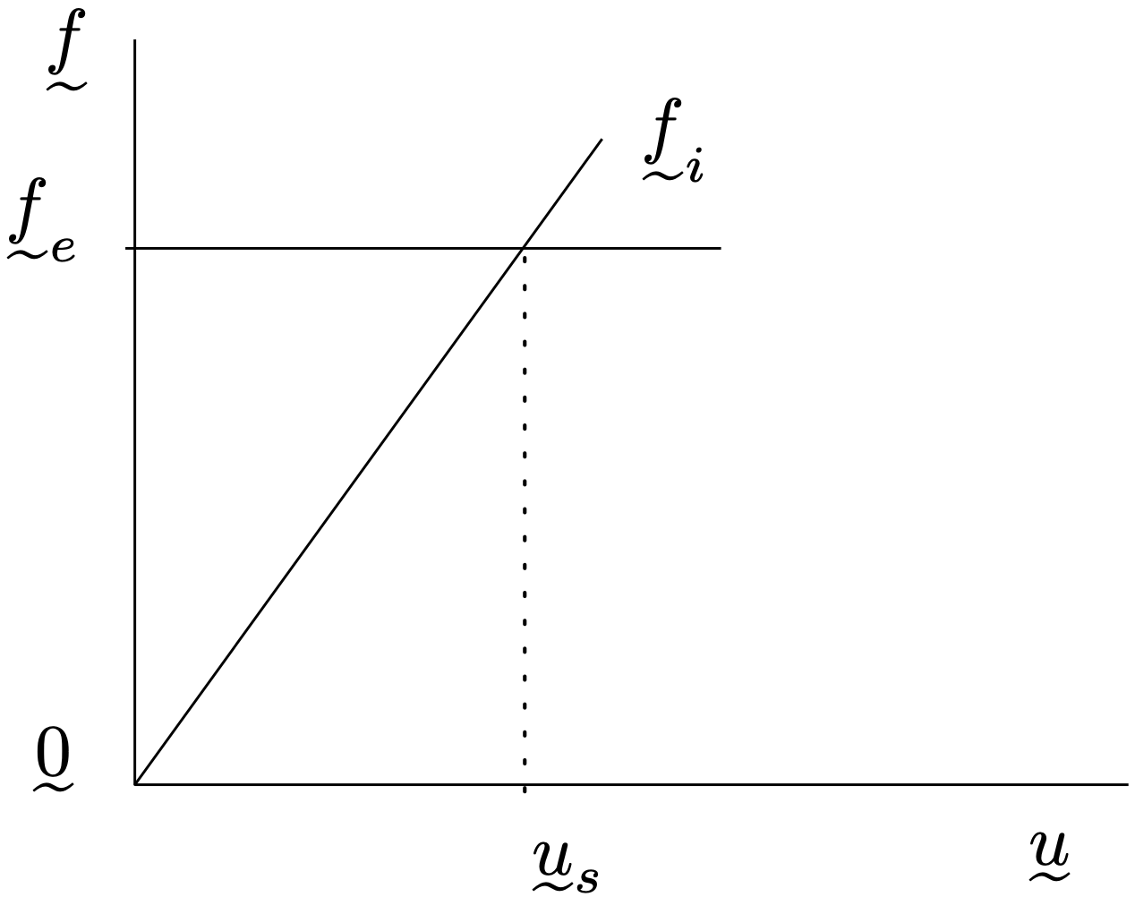
Fig. 3.22 boundary conditions#
When certain errors have been made during modelling, MARC cannot solve the system. A frequently occurring error message is exit number 2004 (see next section for explanation). Usually the cause is insufficient support of the construction, as a result the construction as a whole or parts thereof can perform a rigid movement, without deformation.
MARC-element 9 : three-dimensional truss
MARC-element 9 is a three-dimensional truss element (JOBS→ELEMENT TYPES→TRUSS/BEAM).
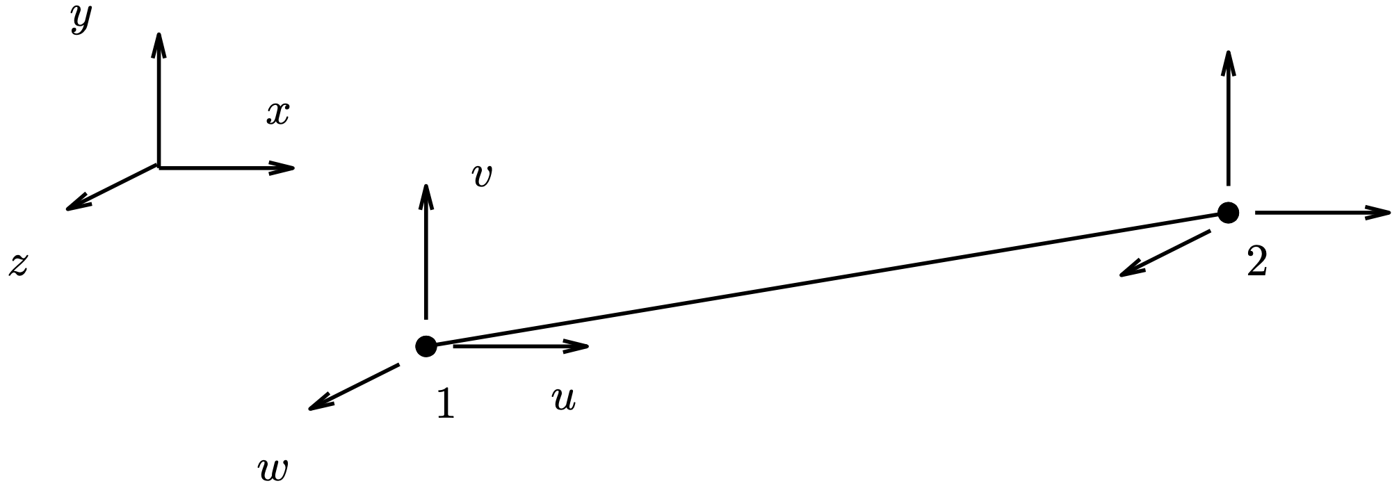
Fig. 3.23 MARC-element 9#
In each node there are three degrees of freedom namely the three displacement components:
| u | = | x displacement | = | displacement_x | = | dof 1 |
| v | = | y displacement | = | displacement_y | = | dof 2 |
| w | = | z displacement | = | displacement_z | = | dof 3 |
The set GEOMETRIC PROPERTIES exists only of the cross-sectional area \(A\).
The set MATERIAL PROPERTIES exists of the elasticity modulus (Young’s modulus) \(E\) and the Poisson’s ratio \(\nu\).
Axial stress and axial strain are calculated in the middle of the element. These quantities can be requested in Mentat and are known already:
| strain_1 | = | uniaxial strain | = | ε |
| stress_1 | = | uniaxial stress | = | σ |
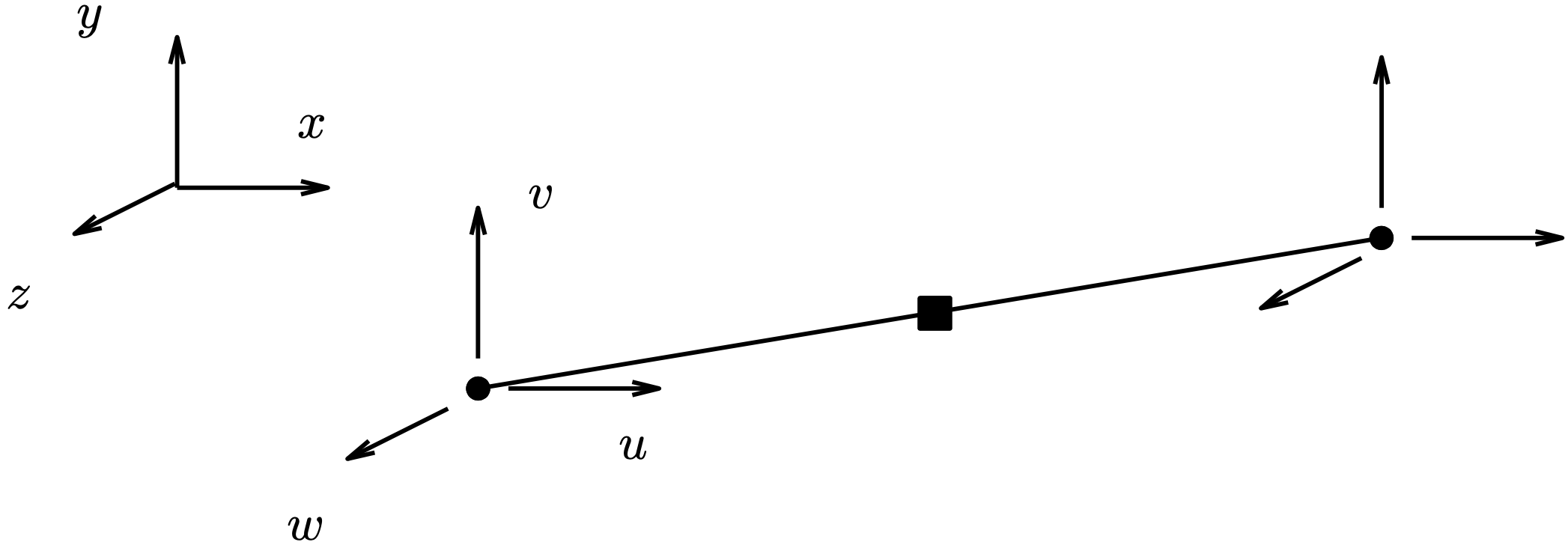
Fig. 3.24 Mentat visualization#
With BEAM VALUES the values can be visualized in colour.
3.3. Two-dimensional truss structures: Analysis#
The model of the construction can now be analyzed. This is done with the finite elements method program MARC. This calculation program can be started from Mentat. That’s what you are going to do via JOBS.
JOBS
RUN
SUBMIT (1)
info
The calculation program MARC is now started and the model is calculated. Infor- mation about the progress of the calculation is given in the (RUN) menu. The word ”working” appears in the status menu.
info
When MARC gives the status ”ready”, the calculation is finished. If everything went well, the (RUN) menu will give exit number \(3004\). Unfortunately sometimes, not everything goes well. Mistakes are made during modelling. MARC responds to this with an error message and the nature of the error is indicated by a exit number. The comment that comes with this code (EXIT MESSAGE) is usually very cryptic or is simply incomprehensible. However, if you have gained some experience with the package, you will notice that the same error codes often return. What also soon becomes clear is where the mistake should be found. The following are a number of common error codes and some indication of the error.
3004 = Fine. The calculation has been successful. This does not imply that the results are good.
13 = MARC does nothing at all. The input is incomplete or so wrong that a calculation cannot even be started. An output file in this case frame1_job1.out will however be written to the hard drive of the computer. With an editor or via the OUTPUT FILE button, this file can be searched for the word error to obtain information about the error(s) in the created model.
2004 = The calculation is aborted because the system-node equations cannot be solved. Usually, this is because the model can deform or move without the need for forces. So check with SWEEP that all nodes are connected to each other and check whether the movement is suppressed as a rigid body.
1005 = When this error message occurs, incorrect or insufficient geometry parameters have been defined. This happens, for example, when one wants to make a model of truss elements and chooses beam elements instead. When the element type is not specified at all for two-dimensional elements, Mentat automatically chooses element number 52, but this is a beam element.
If then everything has gone right after some time, there are, in the directory where
you performed the calculation, four files:
frame1_job1.dat = MARC input file (written by Mentat)
frame1_job1.log = information in the process of the simulation
frame1_job1.out = the alpha-numeric output file
frame1_job1.sts = summary of the .log-file
frame1_job1.t16 = binary file with results for Mentat
The results of the calculation can now be viewed with Mentat. Before doing so, the following section first briefly explains what exactly has been calculated.
3.4. Two-dimensional truss structures: Results#
Let’s assume everything went OK and we can have a look at the results.
info
You select in the main menu RESULTS. The results of the simulation are written in the file with extension .t16 (or .t19). When MARC is started from Mentat, the file frame1_job1.t16 can directly be opened via:
RESULTS
file → open default
(Fill view)
(DEFORMED SHAPE)
DEFORMED \(\&\) ORIGINAL
info
The distortion is displayed, but there is nothing to see, because the distortions are very small. You can do something about that.
(DEFORMED SHAPE) SETTINGS
(DEFORMED SCALING) SETTINGS ● Automatic
info
The real distortion is now scaled up with a (FACTOR) mentioned in the menu.
MODEL PLOT
info
The axial stress (Comp 11 of Stress) in the truss element can be indicated with colour codes. NB: 11 is one-one and not eleven.
(SCALAR PLOT) SCALAR
● Comp 11 of Stress
● OK
(SCALAR PLOT)
BEAM CONTOURS
info
The colours do not give the exact numerical value of the stress because there are certain averaging procedures applied.
Reading the exact value of the normal stress in a truss element can be done as
follows.
(SCALAR PLOT)
NUMERICS
ISOLATE
(ISOLATE ELEMENT) ADD
select element (End list)
info
The value of the stress can now be read in the two nodes between which the element is located. A positive stress is a tensile stress, where a negative value indicates compressive stress. Several elements may be selected simultaneously. However, the specified elements may not be adjacent to each other, because average node values appear again.
info
When we have sufficiently studied the results, it is possible that we come to the conclusion that the model needs to be adjusted. The file frame1_job1.t16 must first be closed, after which the model file frame1.mud can be opened and modified. In order to remove the possibly still present colour bar, you can enter the menu
(SCALAR PLOT) →→ OFF.
file → close
info
Re-opening of the model file (frame1.mud) takes place immediately when the \(^*\).t16-file is closed. If this does not happen, it can still be opened via file in the main navigation menu. If we are done, we can exit Mentat.
file → exit
3.5. Three-dimensional truss structures#
The truss structure that we are going to model is a simple model of the frame to which a basketball net is attached (see the figure on the next page). The truss structure is loaded by a dunking basketball player.
The construction is made up of two different truss elements. The first is a corner and the second a simple strip profile. The cross-sections are shown in the figure below. Because we assume that the truss elements are only axially loaded, the actual shape of the cross-section is not important. For the stiffness - the resistance to deformation - the surface of the cross-section is essential. The values are:
Both profiles are made of steel. The material properties are:
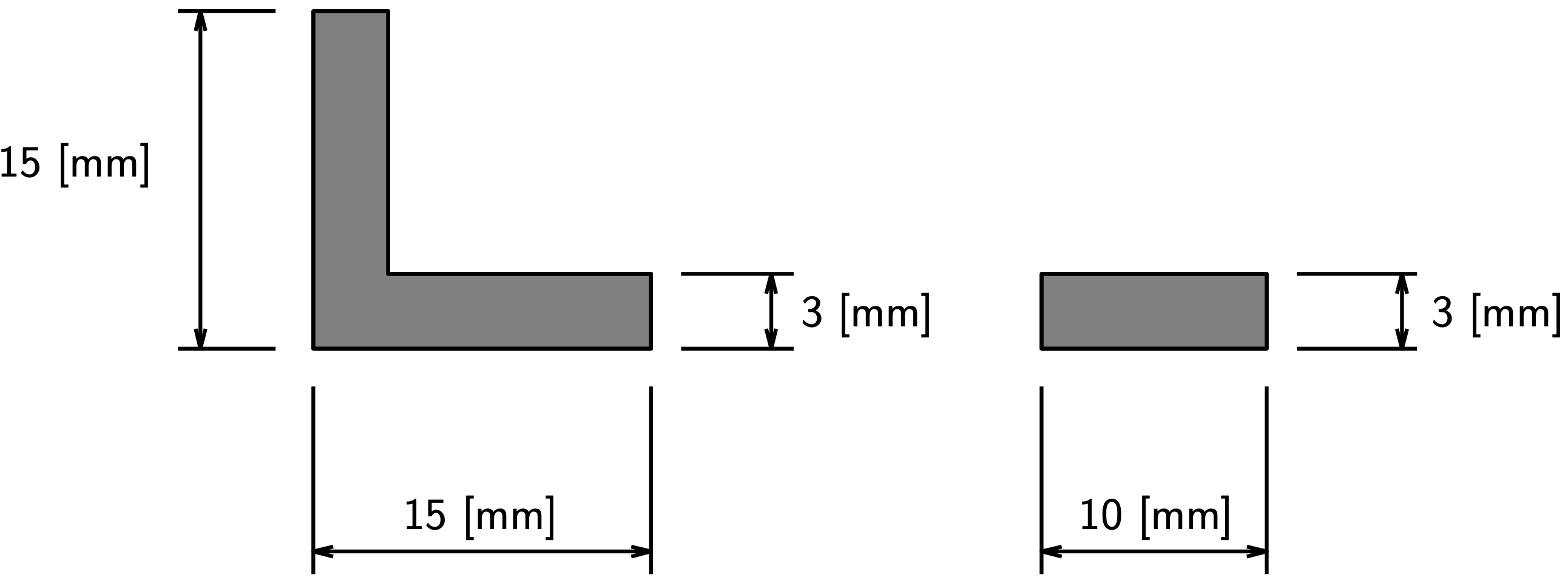
Fig. 3.25 Three-dimensional truss structure#
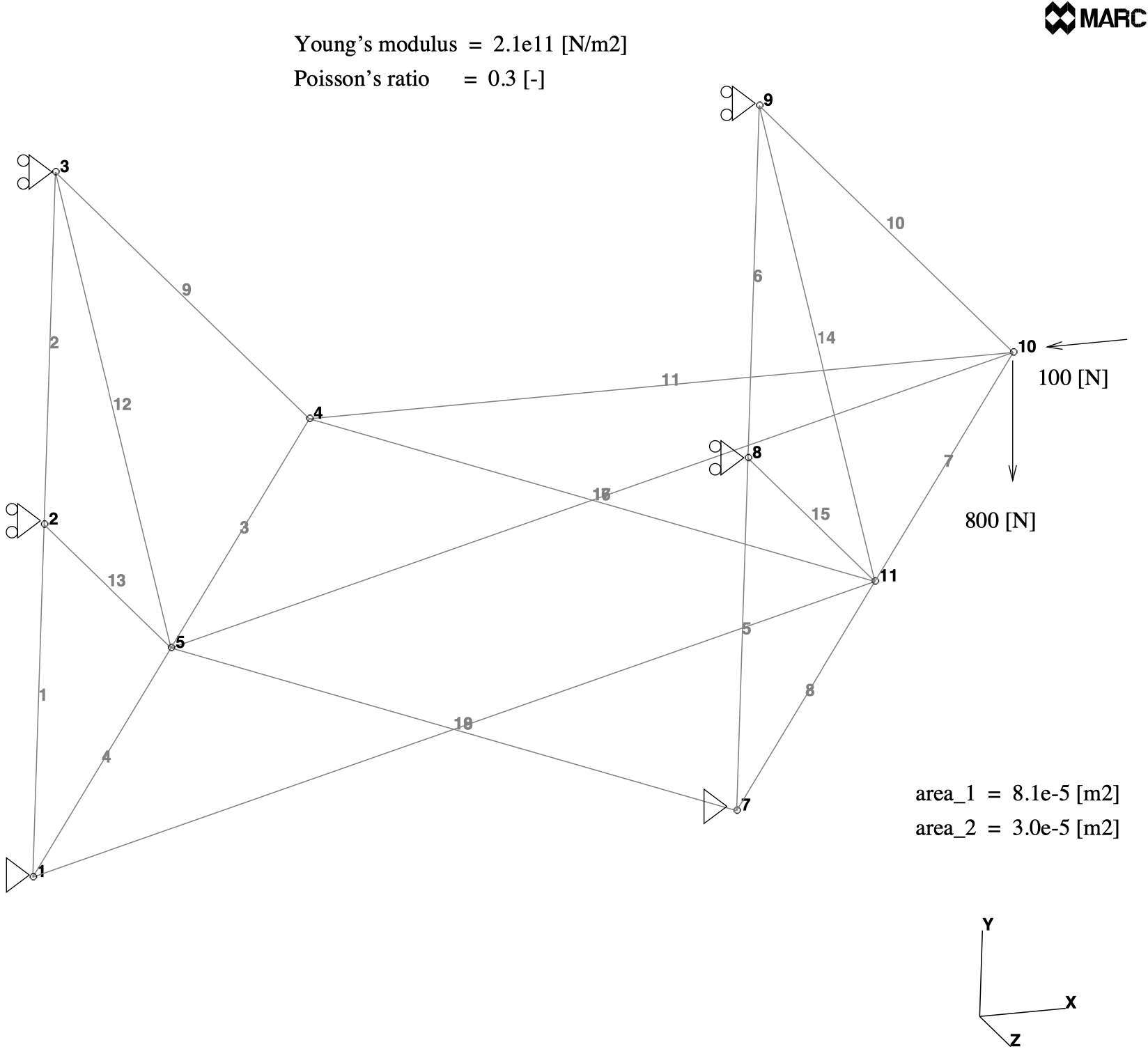
Fig. 3.26 Mentat configuration#
3.5.1. Modelling#
GEOMETRY \(\&\) MESH
info
We start in GEOMETRY \(\&\) MESH and enter the coordinates of some of the points.
GEOMETRY \(\&\) MESH (Basic Manipulation)
(POINTS) ADD
Enter point coordinates (\(X\)): 0, 0, 0
Point added
Enter point coordinates (\(X\)): 0.3, 0, 0
Point added
Enter point coordinates (\(X\)): 0.3, 0.3, 0
Point added
Enter point coordinates (\(X\)): 0, 0.3, 0
Point added
Enter point coordinates (\(X\)): 0, 0.3, 0.3
Point added
Enter point coordinates (\(X\)): 0.3, 0.3, 0.3
Point added
(Fill view)
info
We change the view (rotate) and display the labels of points and curves.
 (Rotate positive x)(2x)
 (Rotate positive y)(2x)
(Fill view)
| view | → | plot control | → | points | (SETTINGS) | → | ☑ labels | → | OK |
| → | curves | (SETTINGS) | → | ☑ labels | → | OK | |||
| → | OK | ||||||||
info
Now we create the curves (straight lines) between the already defined points.
(CURVES)
LINE
(CRVS) ADD
Enter line points: 1, 4
Curve added
Enter line points: 4, 5
Curve added
Enter line points: 5, 1
Curve added
Enter line points: 2, 3
Curve added
Enter line points: 3, 6
Curve added
Enter line points: 6, 2
Curve added
Enter line points: 5, 6
Curve added
info
The truss elements are : LINE(2) First some curves are subdivided with CONVERT , successively the elements are added.
(ELEMENTS)
LINE(2)
CONVERT (Operations)
(CONVERT)
CURVES
DIVISIONS
Enter the number of convert divisions 2
CONVERT
Enter convert curve list: 1, 3, 4, 6, #
GEOMETRY \(\&\) MESH (Basic Manipulation)
(ELEMS) ADD
Enter element node (1): 3, 4
Element added
Enter element node (1): 9, 10
Element added
Enter element node (1): 10, 4
Element added
Enter element node (1): 3, 5
Element added
Enter element node (1): 5, 2
Element added
Enter element node (1): 9, 11
Element added
Enter element node (1): 11, 8
Element added
Enter element node (1): 4, 11
Element added
Enter element node (1): 5, 10
Element added
Enter element node (1): 5, 7
Element added
Enter element node (1): 1, 11
Element added
info
With view → plot control points and curves are made invisible. Elements of curves have to be ”detached” such that they are displayed as ”black”. Coinciding nodes are joined to one. Watch in the Mentat commando-window what is being done.
SWEEP (Operations)
(SWEEP) ALL
(REMOVE UNUSED) NODES
(REMOVE UNUSED) POINTS
info
The geometric properties of the truss elements are then added. In this case, that is only the cross-sectional area. This quantity has a different value for two groups of truss elements.
GEOMETRIC PROPERTIES
NEW (STRUCTURAL)
3-D
TRUSS
PROPERTIES
Cross Section Area: 8.1e-5
OK
(ELEMENTS) ADD
OK
Enter geometry add element list: 1, 2, 3, 4, 5, 6, 7, 8, 9, 10, 11 (End list)
NEW (STRUCTURAL)
3-D
TRUSS
PROPERTIES
Cross Section Area: 3.0e-5
OK
(ELEMENTS) ADD
OK
Enter geometry add element list: 12, 13, 14, 15, 16, 17, 18, 19 (End list)
info
Hereafter the material properties, i.e. the Young’s modulus and the Poisson’s ratio, are defined.
MATERIAL PROPERTIES
NEW
STANDARD
STRUCTURAL
Young’s Modulus: 2.1e11
Poisson’s Ratio: 0.3
OK
(ELEMENTS) ADD
Enter add material element list: (All existing)
info
The boundary conditions are prescribed last. The figure of the truss structure shows which nodes are attached to the fixed world. The forces are also prescribed.
BOUNDARY CONDITIONS
NEW (STRUCTURAL)
FIXED DISPLACEMENT
PROPERTIES
☑ Displacement X
☑ Displacement Y
☑ Displacement Z
OK
(NODES) ADD
Enter add apply node list: 1, 7 (End list)
NEW (STRUCTURAL)
FIXED DISPLACEMENT
PROPERTIES
☑ Displacement X
☑ Displacement Z
OK
(NODES) ADD
Enter add apply node list: 2, 3, 8, 9 (End list)
NEW (STRUCTURAL)
POINT LOAD
PROPERTIES
☑ Force X
Enter value for x: -100
☑ Force Y
Enter value for y: -800
OK
(NODES) ADD
Enter add apply node list: 10, (End list)
info
Further speculation of elements and load is now being done in JOBS
JOBS
NEW
STRUCTURAL
info
The construction considered here is three dimensional. This must be specified in the menu PROPERTIES → ANALYSIS DIMENSION. The load on the construction can be set in PROPERTIES → INITIAL LOADS composed of the defined boundary conditions. If they are already selected, we obviously do not have to do anything. The desired calculation results to be viewed afterwards must be entered in PROPERTIES → JOB RESULTS and are selected from a large number of options. We choose Stress and Total Strain.
PROPERTIES
(ANALYSIS DIMENSION)
3-D
INITIAL LOADS
☑ apply1, ☑ apply2, ☑ apply3
OK
JOB RESULTS
(AVAILABLE ELEMENT TENSORS)
☑ Stress
☑ Total Strain
OK
OK
info
At an earlier stage we opted for line elements. However, the MARC program has a number of line element types. We choose here element no. 9.
ELEMENT TYPES (ELEMENT TYPES)
(ANALYSIS DIMENSION) (ELEMENT TYPES)
3-D
TRUSS/BEAM
TRUSS 9
OK
Enter element list: (All existing)
info
We now save the model
| file | → | save as | → | File name: basket1 | → | SAVE |
3.5.2. Analysis#
Analysis of the model is done directly via Mentat.
For running MARC from Mentat we go to JOBS.
JOBS
RUN
SUBMIT (1)
info
MARC is now started and the model is calculated. The (RUN) menu provides information about the progress of the calculation. The word ”working” appears in the status menu. When the status indicates ”ready”, the calculation is finished. If everything went well, the (RUN) menu displays exit number 3004. The results of the calculation can now be viewed with Mentat.
3.5.3. Results#
Let’s assume everything went according to plan.
info
We select in the main menu RESULTS. The results of the calculation of MARC are written to files with the extension .t19 or .t16, which are read by Mentat.
RESULTS
file → open default
(Fill view)
(DEFORMED SHAPE)
DEFORMED & ORIGINAL
(DEFORMED SHAPE) SETTINGS
(DEFORMED SCALING) ● Automatic
info
The axial stress (Comp 11 of Stress) (11 = one-one) in the truss elements can be acquired in the following way.
MODEL PLOT
(SCALAR PLOT) SCALAR
● Comp 11 of stress
OK
(SCALAR PLOT)
NUMERICS
ISOLATE
(ISOLATE ELEMENT) ADD
select element (End list)
info
The value of the stress can now be read at the two nodes between which the element is located. A positive stress value is known as tensile stress, with a negative value being compressive stress. Multiple elements may be selected simultaneously. However, the specified elements must not be adjacent to each other, because then again average node values appear.
info
We can now exit Mentat.
| file | → | exit |
3.6. Exercises#
In this section some truss structures are two- other are three-dimensional. More than the deformation of the truss structures, the axial stress in each truss element is of great important. Especially compressive stresses are a limiting factor. When in a truss element the compressive stress has reached a certain critical value the truss element will buckle and the structure will collapse.
3.6.1. Two-dimensional portal#
In the figure below a two-dimensional portal is drawn. Its dimensions (in meters) are given in the figure. All non-indicated dimensions must be estimated by your own discretion. (Hint: inter sections of curves can be determined with the tab GEOEMETRY & MESH → INTERSECT (Operations).)
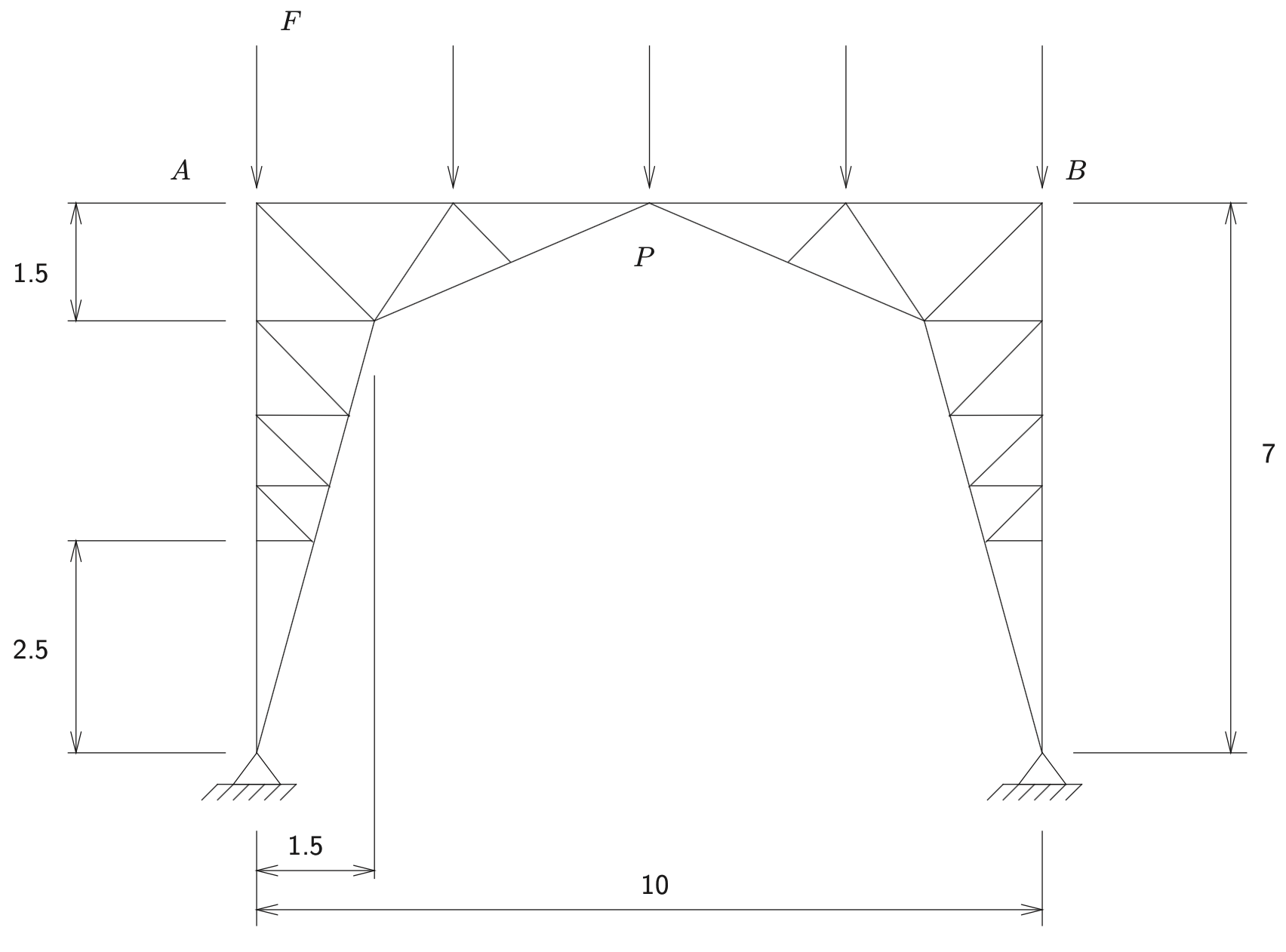
Fig. 3.27 Truss of two-dimensional portal.#
All truss elements have a square cross section as drawn in the Fig. 3.28 below. In the table the dimensions of the ”outer” truss elements (OUEL) and ”inner” truss elements (INEL) are indicated in millimetres (mm)[1].
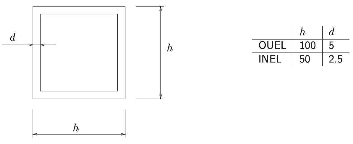
Fig. 3.28 Truss square cross sections.#
All truss elements are made of Aluminium and the material properties are:
The portal is loaded vertically, where the direction is indicated in the figure. All indicate forces are equal to: \(F = 1000\) [N].
Check if it is sufficient to model only half of the construction. Which boundary conditions must then be defined in point P? Is it possible to omit one or more truss elements? Do you recommend this is view of buckling?
3.6.2. Climbing tower#
At the TU premise, close to the gym, a climbing tower is located. We will model a similar tower here as a space frame. The tower is outlined and relevant dimensions are given in the figure below (in meters).
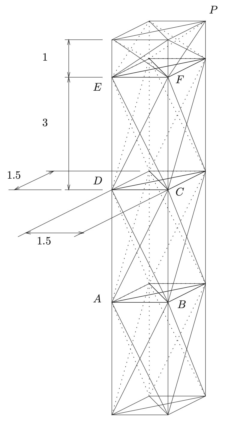
Fig. 3.29 Climbing tower truss structure.#
When modelling the space frame make use of duplication of certain sections (truss elements with ele- ment properties) (GEOEMETRY & MESH → DUPLICATE (Operations)).
The cross sections of the horizontal and vertical truss elements (HVS) and of the diagonal truss elements (DNS) are shown in the Fig. 3.30 below. The indicated dimensions are in millimetres.
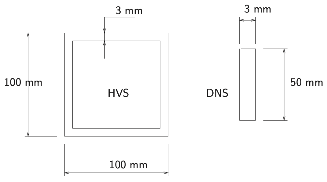
Fig. 3.30 Truss square cross sections.#
The truss elements are made of Aluminium with the following material properties:
The tower is used as a climbing tower, where the weight of several climbers (max. 1000 kg) is evenly distributed over the points \(A\), \(B\), \(C\) and \(D\) or the points \(C\), \(D\), \(E\) and \(F\).
Calculate the deformation and stresses in the truss elements of the construction.
The tower can also be used as a mounting point for a cable that is anchored in the ground at the other end. Along this cable a person can - with a pulley - slide down to the ground (zip line). Suppose the cable is attached between points P and Q. The person sliding down weighs 80 [kg]. Suppose the cable is distorted as shown in the Fig. 3.31 below.
Calculate the force in point P of the tower and analyse the truss structure.
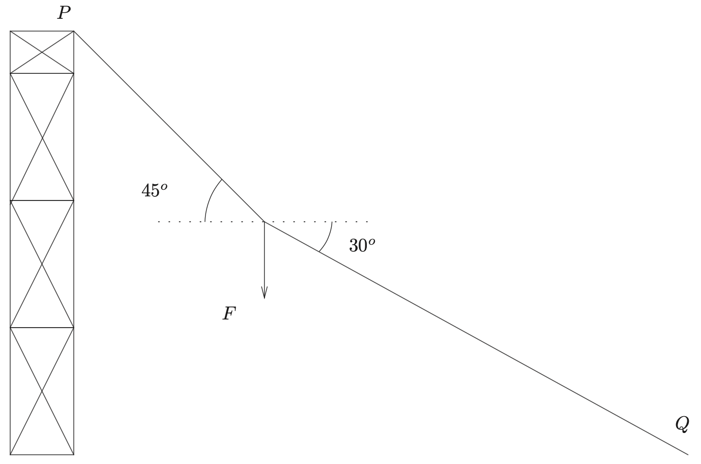
Fig. 3.31 Sliding person truss structure.#
3.6.3. Construction crane#
The boom of a construction crane is outlined in Fig. 3.32 below. Dimensions are indicated in the figure (in meters). Dimensions not specified must be estimated.
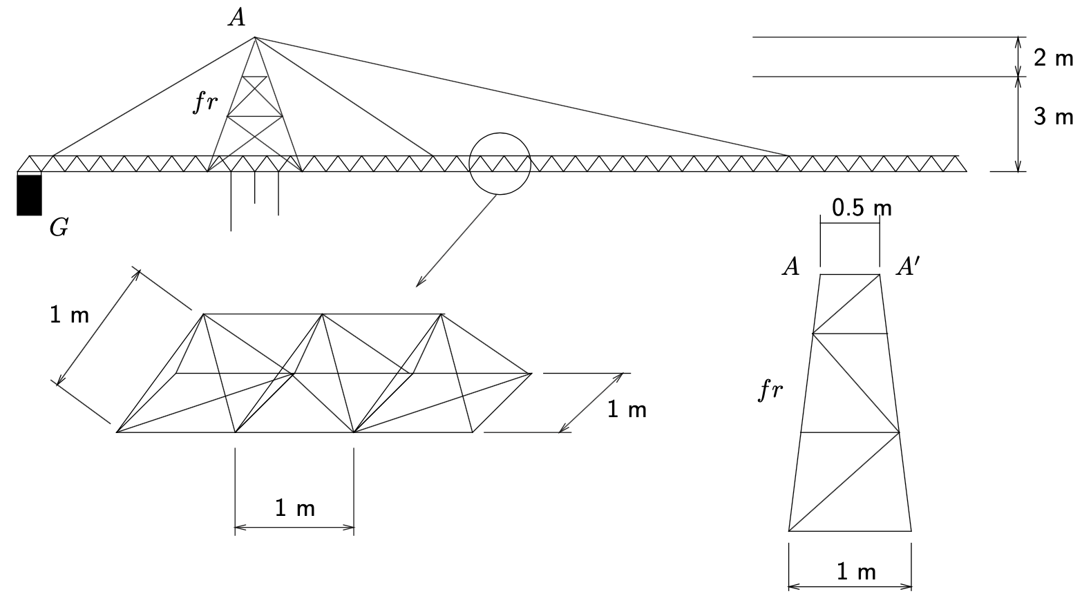
Fig. 3.32 Construction crane truss structure.#
The horizontal truss elements of the boom are hollow cylindrical tubes with an outer diameter of 100 mm and a wall thickness of 8 mm. The diagonal truss elements are also hollow cylindrical tubes with a outer diameter of 70 mm and a wall thickness of 5 mm. The frame, \(fr\), is also built from such tubes. The front view is drawn in the figure. Between the points \(A\) and \(A`\) of the frame and the boom there are cables that can be modelled as solid cylindrical bars with a diameter of 10 mm.
All tubes and bars are made of steel with the following material properties:
The contra weight \(G\) has a mass of 5000 kg and is connected to the boom with cables.
Analyse the construction crane for various loads, located at different positions along the boom.