
5. Deformation of trusses. Statically indeterminate systems. The finite element method#
Book: Section 3.4 (excluding subsections 3.4.2 and 3.4.3),introduction Chapter 4 and section 4.2 (excluding subsections 4.2.2 and 4.2.3).
5.1. Deformation of statically determinate systems#
For each member of a statically determinate truss under isothermal conditions (constant temperature) the following stress-strain relation applies:
Here, \(T\) is the member force, which is positive (negative) under tension (compression). If the strain is small in all members, it is allowed (as an approximation) to apply equilibrium of forces in each joint using the undeformed geometry. This allows all forces in the system to be determined without knowing the deformation of the truss.
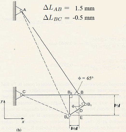
In order to determine the displacement of a joint (node), we have to satisfy compatibility of strains. In other words: the displacements of the joints must be such that the members are still connected after the deformation. For a truss consisting of only two members, satisfying compatibility of strains is rather straightforward. It is explained on the pages 123-126, first in an exact way and then in an approximate way (Figure 3.13b). The approximate approach is what we will be using from now on for exercises and exam questions.
Deformation of a truss having multiple members is more difficult to analyse by analytical methods and we will be using the finite element method instead (i.e. Marc/Mentat in this course). By default Marc/Mentat uses a geometrically linear approach. This means that equilibrium of forces is applied with respect to the undeformed geometry and that expressions for the strains in the members are linearised and only valid for small displacements and rotations. The solutions are therefore also only valid if the displacements and rotations are very small with respect to the global dimensions of the undeformed structure. From a practical point of view, this means that the deformation is hardly noticeable with the naked eye.
If deformation and rotation of the structure become large the geometrically linear approach is insufficient and the change in geometry needs to be taken into account for the equilibrium of forces. In Marc/Mentat the option “large displacements” needs to be used. Also, if the strains become large the linear elastic material behaviour given by Hooke’s law is insufficient and needs to be replaced by a nonlinear material law (sometimes called physically nonlinear). In both cases, geometric and material nonlinearity, it means that the equations to solve are nonlinear in the displacements. Solving these equations requires a special approach, where the load is applied in several small steps (increments) and the equations are solved for each load step using iteration.
Sections 3.4.2 and 3.4.3 are not part of the exam
Section 4.1 is not part of the exam. Instead the following short text is a simple replacement without equations, sufficient to use the program Marc/Mentat in a meaningful way.
The finite element method for statically determinate and indeterminate trusses
In the finite element method the joints in the truss are called nodes. In each node three displacement components (in \(x\), \(y\) and \(z\) direction) and three force components are defined. The strains in the members can be expressed in terms of the displacements of the nodes, assuming the members remain connected to the nodes after deformation (compatibility). Using Hooke’s law, the stresses and normal forces in the members can be expressed in the displacements of the nodes. After substituting these expressions into the equilibrium of forces of all the nodes, a set of equations expressed in the displacements of the nodes is obtained. Note, that the external forces (dynamical boundary conditions) end up in the right-hand side of the system. In nodes where a displacement component is suppressed or imposed (kinematic boundary conditions), unknown reaction forces are still present. These unknown forces can be discarded by substituting the value of the imposed displacement and simply discarding the corresponding equilibrium equation from the set of equations. In this way, a set of linear equations is obtained for the unknown degrees of freedom: the unknown displacement components. Since the unknowns in the linear system are displacements (not forces), this is called the displacement method.
Displacement method:
Displacements of the joints/nodes are the unknowns.
Strains in the members can be expressed in terms of the displacements of the joints/nodes (strain-displacements relations).
Using Hooke’s law, forces can be expressed in terms of the displacements.
Substitution of the force expressions into the equilibrium equations for the joints/nodes leads to a system of equations for the displacements.
Substitute:
Kinematic (essential) boundary conditions: prescribed displacements.
Dynamic (natural) boundary conditions: prescribed external forces.
Omit the equations containing reaction forces.
System of equation in the unknown displacements only.
If the kinematic boundary conditions are such that all rigid body modes are suppressed, the system will be regular and can be solved. If rigid body modes are not sufficiently suppressed, the connectivity of the members is such that the structure is a mechanism, or some members have zero stiffness, the system will be singular and can not be solved. In that case, in Marc/Mentat gives an error message with the number 2004.
After successfully solving the displacements of the nodes, the strains, stresses, normal forces and reaction forces can be computed in a post-processing step.
Note
The displacement method does not differentiate between statically determinate and indeterminate systems and works for both in the same way.
5.2. Other statically indeterminate systems#
Study Examples 4.6 and 4.7, showing typical statically indeterminate problems. Sections 4.2.2 and 4.2.3 are not part of the exam.
Supported rigid bar
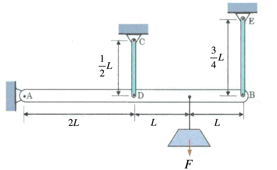
Fig. 5.1 Rigid horizontal bar \(AB\) pinned at \(A\) and connected at \(D\) and \(B\) to vertical rods \(CD\) and \(EB\).#
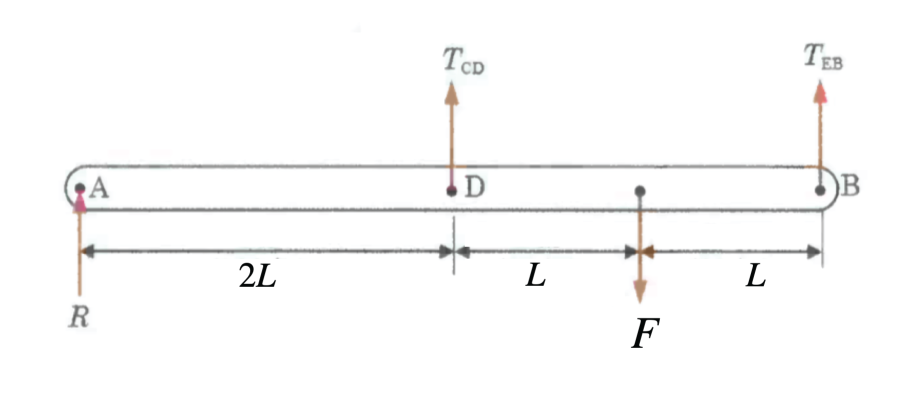
Fig. 5.2 Free-body diagram of bar \(AB\).#
In this problem we have a rigid horizontal bar \(AB\), pinned at \(A\) and tied to the ceiling by two vertical elastic rods at \(D\) and \(B\). A concentrated load \(F\) hangs at the mid-span of the bar. Because there are three unknown support reactions (at \(A\), \(D\) and \(B\)) but only two equilibrium equations for the bar, the system is statically indeterminate. Find the small rotation \(\theta\) of the bar (and thereby the vertical displacements at \(D\) and \(B\)).
Solution
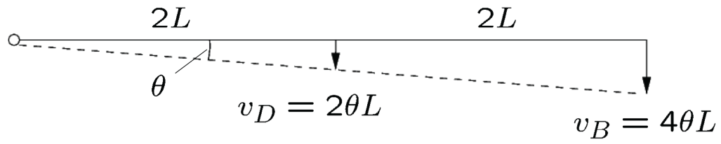
Fig. 5.3 Strain displacement relations.#
The moment balance about the hinge \(A\) must be zero in equilibrium. This gives
\(\displaystyle v_D = 2 L \theta\) and \(v_B = 4 L \theta\) as shown in Fig. 5.3 express the vertical drops of the rod attachment points \(D\) and \(B\) purely in terms of the bar’s small rotation angle \(\theta\).
The Constitutive (force–displacement) relations are
for member \(CD\) and \(EB\) respectively. By substituting the compatibility and constitutive relations into the equilibrium equation, yielding a single equation in the unknown \(\theta\) then finally gives
Also, practice the case where \(k_{CD}\) and \(k_{EB}\) are given (not \(E\), \(A\) and the length of \(CD\) and \(EB\)). This gives
Steel bolt and copper tube
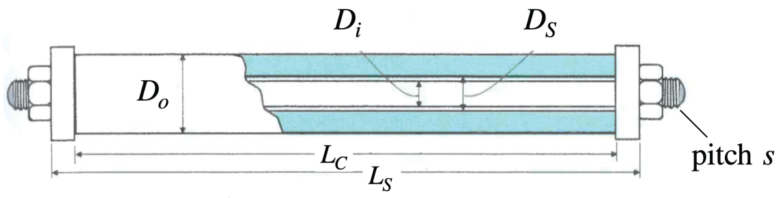
Fig. 5.4 Steel bolt and copper tube#
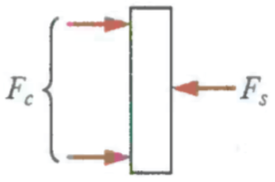
Fig. 5.5 View of forces on the bolt#
The figures Fig. 5.4 and Fig. 5.5 show a simple description of a steel bolt and copper tube where the dimensions and forces present have been provided. Below in figures Fig. 5.6 and Fig. 5.7 The equilibrium and strain displacement relations (compatibility) of the system are visible.
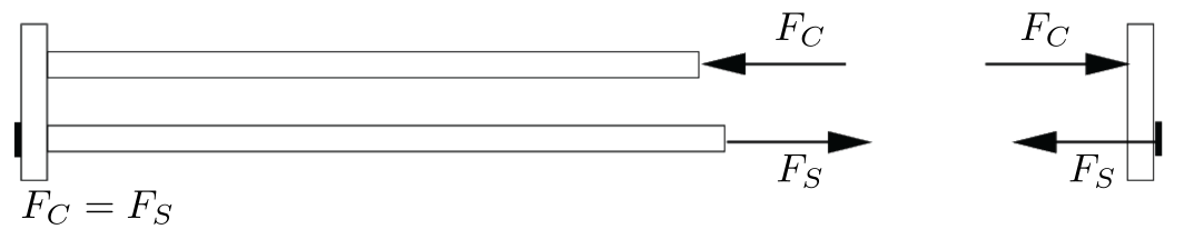
Fig. 5.6 View of forces on the bolt#
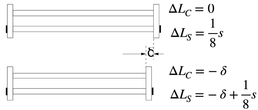
Fig. 5.7 View of forces on the bolt#
Solve for the joint shortening \(\delta\), the common axial force \(F\) (with \(F_S=F_C\)) induced by the \(\frac{1}{8}\)-turn advance \(\frac{s}{8}\), and the resulting stresses \(\sigma_S\) and \(\sigma_C\) in the steel bolt and copper tube.
Solution
The constitutive relations for this system are found to be
The solution strategy is to follow go from
Strain-displacement \(\implies\) Constitutive relation \(\implies\) Equilibrium.
This provides us with enough information to find
and with \(\delta\) we can find \(\displaystyle \implies F_S, \ F_C, \ \sigma_S, \ \sigma_C\).
5.2.1. Some typical examples#
For statically indeterminate systems the procedure is as follows. First, express the forces in the system in terms of the unknown displacements, using the strain-displacement relations (compatibility) and the stress-strain relations. Then substitute the force expressions into the equilibrium of forces. From the resulting equations the unknown displacements can be solved. Finally, the strains, stresses and forces can be computed. See Example 4.4. This procedure for solving statically indeterminate systems very much resembles the displacement method as used in the finite element method.
Results derived in this section:
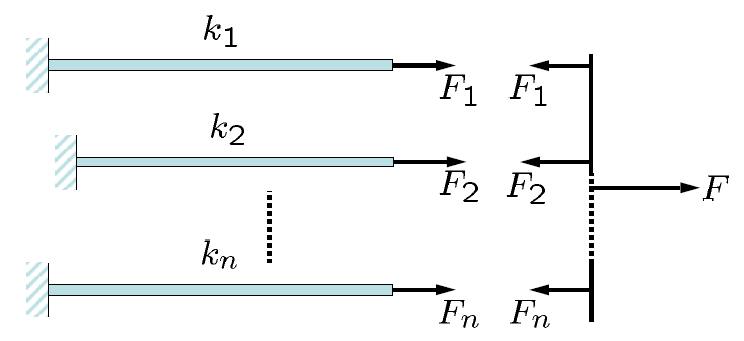
For \(n\) elastic elements in parallel, where \(k_i\) with \(i = 1,2,...,n\) are the individual stiffnesses of the elements, the total stiffness \(k\) is given by \(k = \sum_{i = 1}^{n} k_i\). See Example 4.4.
Chest expanders
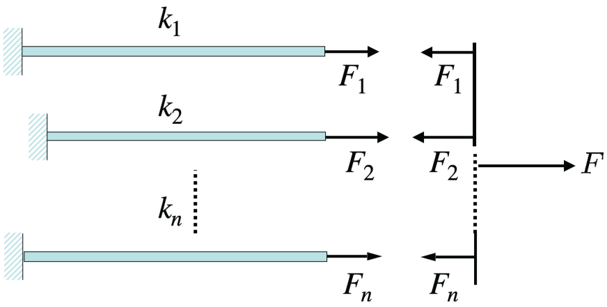
Fig. 5.8 parallel spring arrangement#
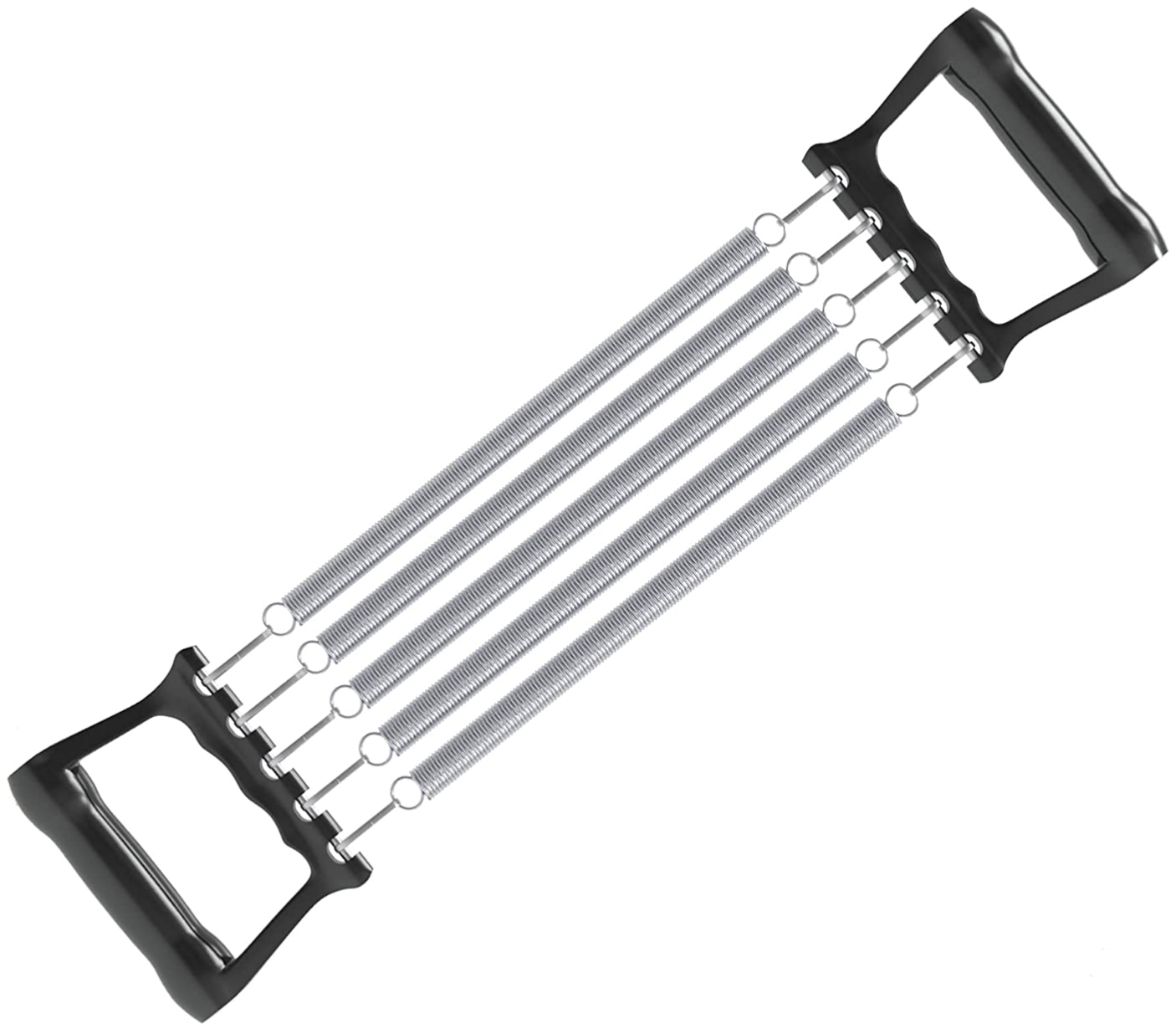
Fig. 5.9 Synonymous chest expander system#
For the parrallel spring arrangement visible in Fig. 5.8 \(n\) springs are parallel to eachother with
for the spring extension and with this
for the total net force in the entire system. With \(n\) elements in the series we can define \(k\) by
For a parallel circuit for a Force \(F_i\) we use the defenition
This parallel spring system that we worked out above has the same type of dynamics as a chest expander as described by Fig. 5.9.
For \(n\) elastic elements in series, where \(k_i\) with \(i = 1,2,...,n\) are the individual stiffnesses of the elements, the total flexibility \(f=1/{k}\) is given by \(f = \sum_{i = 1}^n f_i\) where the individual flexibilities are \(f_i=1/{k_i}\) with \(i = 1,2,...,n\). See Example 4.6.
Springs in series
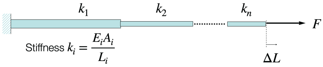
Fig. 5.10 parallel spring arrangement#
For in series spring arrangement visible in Fig. 5.10 \(n\) springs are linearly in series with different spring constants that run with stiffness
The forces are described by
The total displacement equals the sum of all of the displacemnts of the individual springs described as
using \(\displaystyle \frac{1}{k}=\sum_{i=1}^n \frac{1}{k_i}\). Now the necessary tools have been established to find the total flexibility
5.3. Quiz#
5.3.1. Question 1#
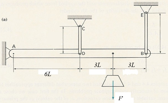
Fig. 5.11 Figure for question below.#