
3. Stress and strain#
Book: Sections 1.3 to 1.5.
3.1. The concept of stress#
Note
Three different definitions for the stress \(\sigma\) are being used here:
The mean (normal) stress in a bar is defined as: \(\displaystyle \sigma = \frac{\text{normal force}}{\text{cross-sectional area}}.\)
The (normal) stress intensity on a small part \(\Delta A\) of the cross-sectional area: \(\displaystyle \sigma = {\Delta F}/{\Delta A}.\)
The local (normal) stress in a point: \(\displaystyle \sigma = \lim_{\Delta A \rightarrow 0} {\Delta F}/{\Delta A} \).
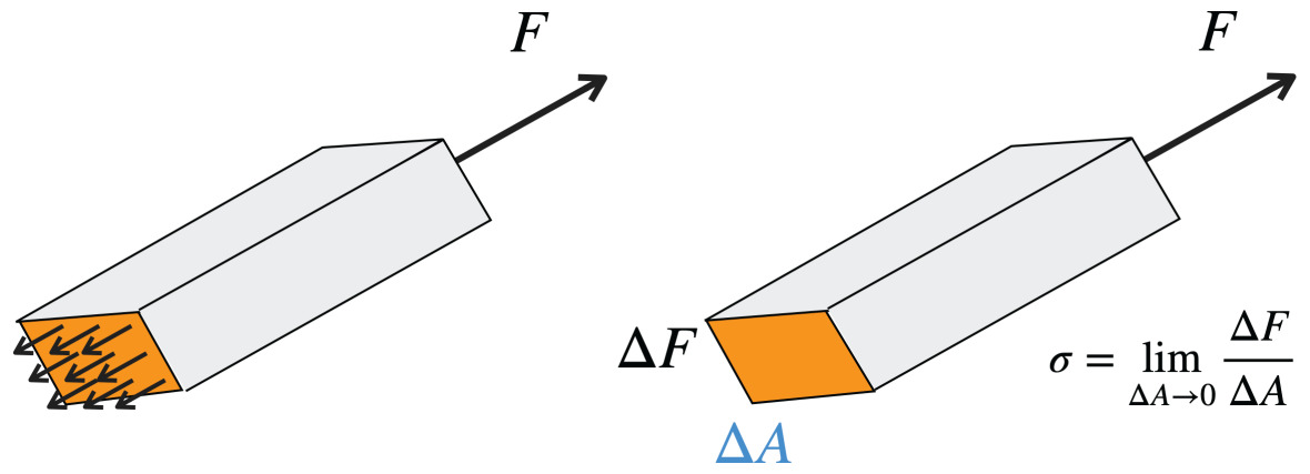
Fig. 3.1 Homogenous normal stress distribution#
If the (normal) stress in every point of the cross-section is the same everywhere, and thus equal to the mean (normal) stress, we say that we have a homogeneous (normal) stress distribution. This is shown in Fig. 3.1 above.
Even in a tensile bar the normal stress distribution is usually inhomogeneous because of end effects. However, at a position sufficiently far from the ends the normal stress distribution can be considered homogeneous if the material itself is homogeneous (Saint-Venant’s principal).
Unit of stress: \(\text{N}/\text{m}^2\) of \(\text{Pa}\) (pascal). Often in megapascal MPa (\(10^6\) Pa) or \(\text{MN} / \text{m} ^ 2\).
The mean shear stress \(\tau\) is defined as the total shear force \(F\) divided by the area \(A\) it is acting on (see Figure 1.15). For the local shear stress \(\tau\) on an infinitesimally small plane in a point, we have again \(\displaystyle \tau = \lim_{\Delta A \rightarrow 0} {\Delta F}/{\Delta A}\). Fig. 3.2 Below shows how shear stress can be visualised on a body. These shear stresses are always tangetial towards the surface.
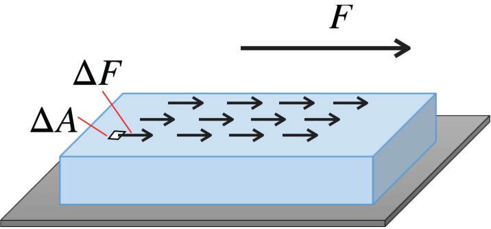
Fig. 3.2 Shear stress on surface of body#
In general, we can define nine different stress components on an infinitesimally small rectangular box at a point \(P\): three normal stress components \(\sigma_1\), \(\sigma_2\) and \(\sigma_3\) (see Fig. 3.3) and six shear stress components \(\tau_{12}\), \(\tau_{21}\), \(\tau_{13}\), \(\tau_{31}\), \(\tau_{23}\) and \(\tau_{32}\). Here, \(\tau_{ij}\) with \(i=1,2\) or \(3\) and \(j=1,2\) or \(3\) in a \(x_1\), \(x_2\), \(x_3\)-coordinate system, are defined as the infinitesimal shear face \(F_\text{s}\) in \(x_j\)-direction divided by the infinitesimally small area normal to the \(x_i\)-axis. The nine stress components are depicted in the figure below:
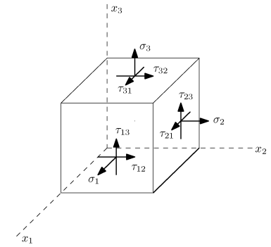
Fig. 3.3 Nine stress components visualised on a cube.#
3.2. Stress concentrations#
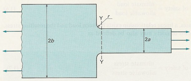
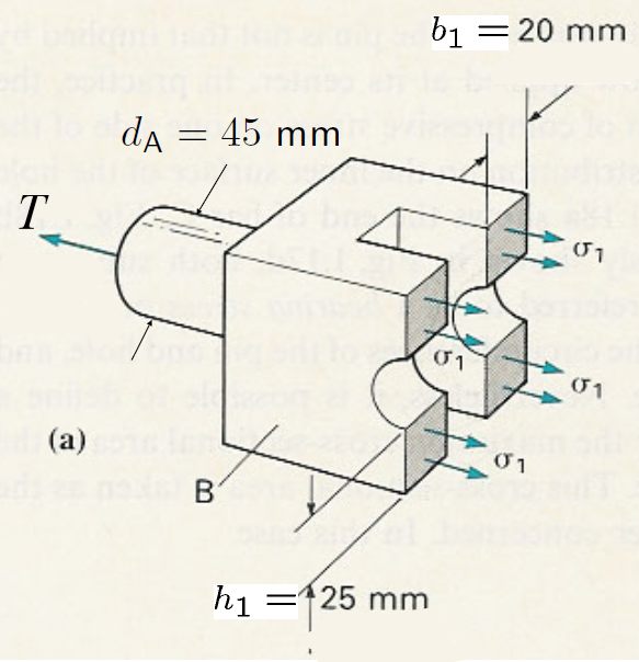
Near circular holes and notches in bars, beams and plates or at sudden changes in cross-sectional area, the local stress will strongly deviate from the mean stress. The ratio between the maximum stress \(\sigma_\text{max}\) and the mean stress \(\sigma_\text{mean}\) is called the stress concentration factor \(K\):
The values of \(K\) for different cases have been tabulated in handbooks (for example by Peterson). Fig. 3.4 below shows an example of stress concentration for a cicular hole relative towards a large plate.
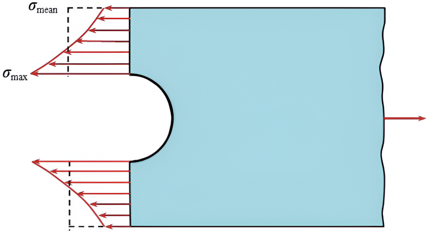
Fig. 3.4 A circular hole in a relatively large plate the factor \(K\) tends to the value 3.#
Every material has a maximum possible tensile stress, the ultimate tensile strength. In order for a structure to not collapse, the local stress in each point of a structure must be smaller than the ultimate tensile strength. Moreover, a factor of safety\(>1\) will be used to define an even lower allowable stress:
Section 1.3.4. in the book give a discussion for an appropriate factor of safety. Below in figures Fig. 3.5 and Fig. 3.6 other examples are given of how stress differ based on shape configuration.
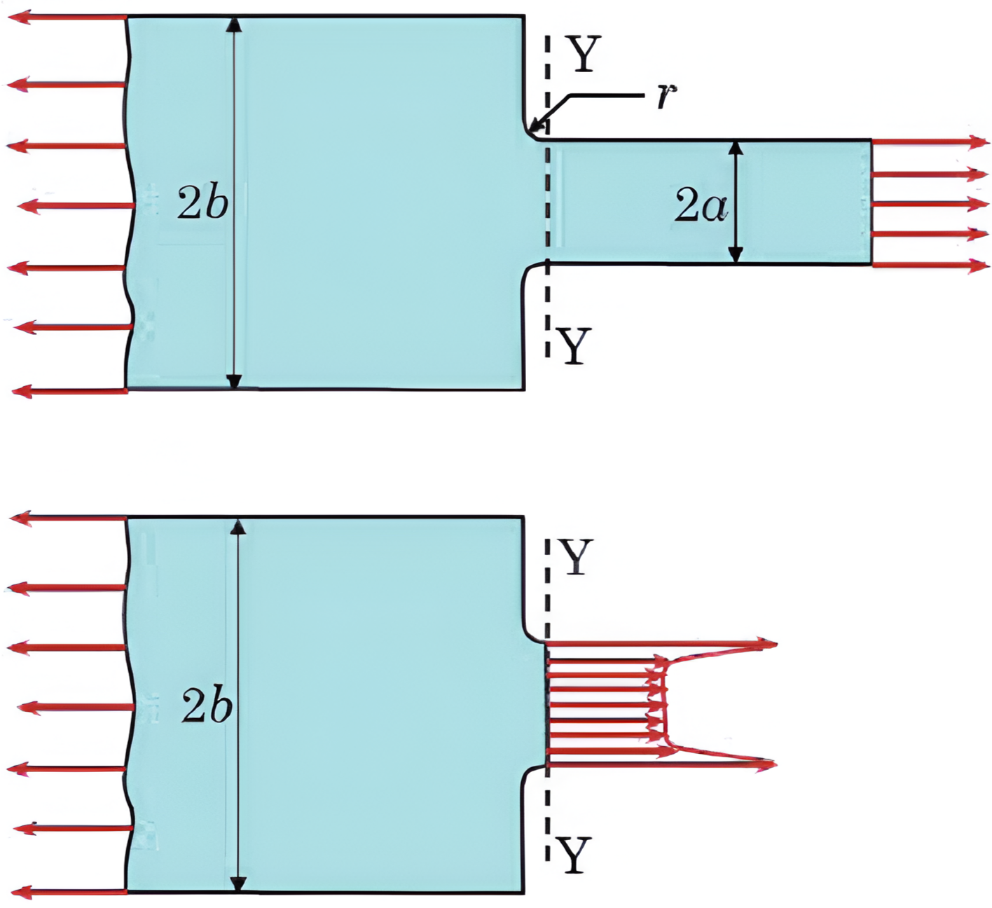
Fig. 3.5 Stress concentration on rectangle with or without narrow slit.#
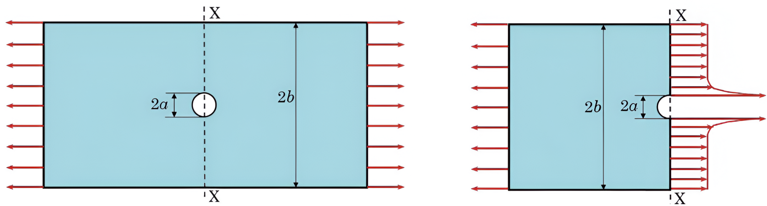
Fig. 3.6 Stress cincetration with Circle in rectangle or on boundary.#
3.3. The concept of strain#
The concept of strain is used to quantify the (local) deformation of the material. Several definitions are possible and some common ones are defined here. Note, that whatever definition is used, strain is always dimensionless.
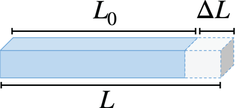
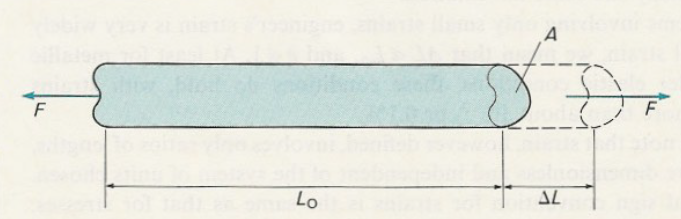
Fig. 3.7 Rectangular prism within relation towards Equation (3.3).#
Fig. 3.7 shows an example of engineering strain, for linear elastic material behaviour the engineering strain [1] or just strain is mostly used, defined by:
Note, that \(e>0\) for extension and \(e<0\) for compression. For elastic deformation of metals we usually have \(|e| < 0{,}001\) or \(|e| < 0{,}1\%\).
For elastic deformation of rubbers, strains will be much larger than for metals and instead of \(e\) the extension ratio \(\lambda\) is commonly used, defined as
For plastic deformation (irreversible deformation) it is common to use the concept of natural strain, defined as:
A measure for the deformation in shear (see Figure 1.23) is the shear strain defined as \(\gamma = \tan(\phi)\). For small deformation we have \(\gamma= \tan(\phi) \approx \phi\) (\(\phi\) in radians). An example is given in Fig. 3.8 below.
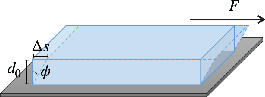
Fig. 3.8 Shear strain on a rectangular prism.#
3.4. The tensile test#
When concidering tensile test some important concepts need to be looked examined. A typical tensile test configuration can be seen in Fig. 3.9
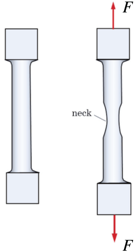
Fig. 3.9 Tensile testing on dog-bone specimen. Clear necking can be seen on the right figure just before breaking.#
The yield point; beyond this point in the stress-strain curve permanent deformation can be detected after removing the load.
The yield strain and yield stress are the values of the strain and stress at the yield point, respectively.
Brittle (opposed to ductile) material behaviour: small (opposed to large) plastic (permanent) deformation at fracture.
Strong (opposed to weak) material: high (opposed to low) ultimate strength.
Stiff (opposed to compliant) material: a steep (opposed to flat) line in the elastic regime of the stress-strain curve. The material stiffness in the lineair elastic regime is characterised by the modulus of elasticity or Young’s modulus \(E\), which is the ratio \(\sigma/e\).
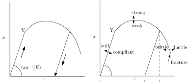
Fig. 3.10 Stress strain curves.#
Note, that the concepts of hard and soft are not applicable to the tensile test (see material science courses).
Below two videos can be seen where either work-hardened copper in the first video or annealed copper in the second video are put under tensile testing.
3.5. The required equations for solving a problem in mechanics#
The required equations for solving a mechanics problem for deformable bodies under static conditions can be divided into three categories:
Equilibrium of forces and moments.
The relations between strains and displacements (compatibility relations).
The stress-strain relation of materials, also called constitutive behaviour.
For statically determinate problems only the first category is needed.
3.6. Additional Videos#
The two videos below by The Efficient Engineer give another perpsective on an introduction to stress and strain and towards understanding Material Strength, Ductility and Toughness. These videos are non mandatory and are purely to give a different persective on the topic.