
6. Bending of beams: moments and forces#
Book: Introduction to Chapter 5, Sections 5.1 and 5.2 (excluding Subsection 5.2.3).
6.1. Bending of beams; moments and forces#
A beam is a slender structural member (i.e. the cross-sectional area is small compared to its length), that can be loaded in lateral direction. This type of configuration can be seen in Fig. 6.1. Like the members of a truss, it can be loaded in axial direction (normal forces), but this will not be considered at first.
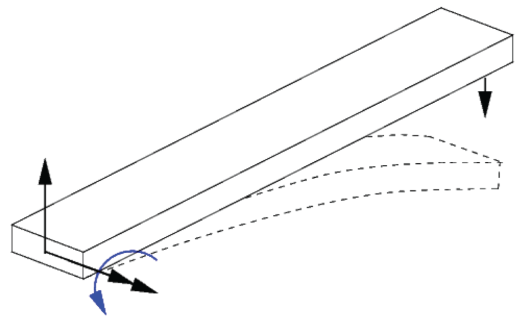
Fig. 6.1 Lateral loaded beam#
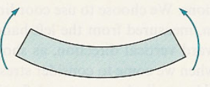
In order to resist lateral loads, (internal) moments and shear forces are created to keep the beam in equilibrium. The moments are created by bending, i.e. the beam becomes curved. In Section 5.1 several practical examples of structures that can be modelled as beams are presented. At first, we only consider two-dimensional beams, i.e. external forces and the bending of the beams is restricted to the \(x,y\)-plane.
In subsection 5.1.1 several support types for beams are given:
- Pinned support
The displacements in \(x\) and \(y\) are constrained and the rotation of the beam is free. As a result, two reaction forces are induced (in \(x\) and \(y\)) and no reaction moment. The graphic Fig. 6.2 below shows an example of this.
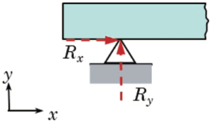
Fig. 6.2 Pinned support#
- Rolling support
The displacement in one direction is constrained. In the direction normal to that, the displacement is free. The rotation of the beam is also free. As a result a reaction force is induced in the constrained direction only. There is no reaction force in the free direction and no reaction moment, i.e. they are zero. Rolling support is sometimes also called sliding support. The graphic Fig. 6.3 below shows an example of this.
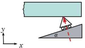
Fig. 6.3 Rolling support#
- Fixed support
The displacements in \(x\) and \(y\) and the rotation are constrained. As a result, two reaction forces (in \(x\) and \(y\)) and a reaction moment are induced. Fixed support is sometimes also called built-in support. The graphic Fig. 6.4 below shows an example of this.
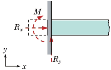
Fig. 6.4 Fixed or built-in support#
A simply supported beam is defined as a beam that only constraints the translational motion as seen in Fig. 6.5.
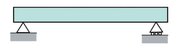
Fig. 6.5 Simply supported beam#
A cantilever is a beam that has fixed support on one side and is fully free on the other. These are examples of statically determinate beams, since the number of unknown reaction forces/moments is equal to the available equilibrium equations (\(=\)three for two-dimensional problems).
Fig. 6.6 shows examples of beams that are statically indeterminate, since the number of unknown reaction forces/moments is larger than three (four and six, respectively).
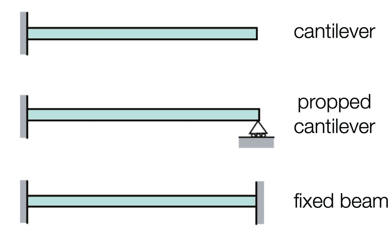
Fig. 6.6 A cantilever, a propped cantilever and a fixed beam.#
In Fig. 6.7-Fig. 6.12 different types of load are shown:
Non-uniformly distributed lateral force as shown in Fig. 6.7.
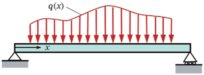
Fig. 6.7 Non-uniformly distributed lateral force system.#
Uniformly distributed lateral force as shown in Fig. 6.8.
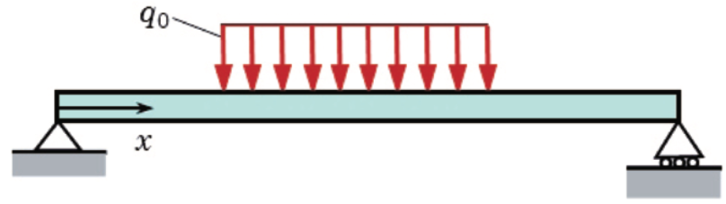
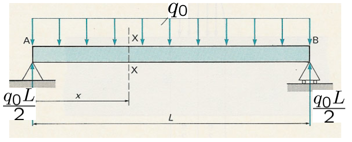
Fig. 6.8 Uniformly distributed lateral force system.#
Concentrated forces (point forces). These are idealisations of non-uniformly distributed forces over a short length scale as shown in Fig. 6.9.
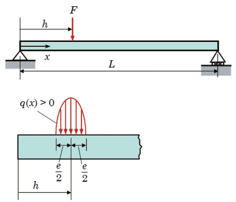
Fig. 6.9 Examples of concentrated forces.#
Concentrated couples. These are idealisations of two opposing non-uniformly distributed forces over a short length scale, where the resulting force is zero, but the moment is not. Examples are shown in Fig. 6.10-Fig. 6.12.
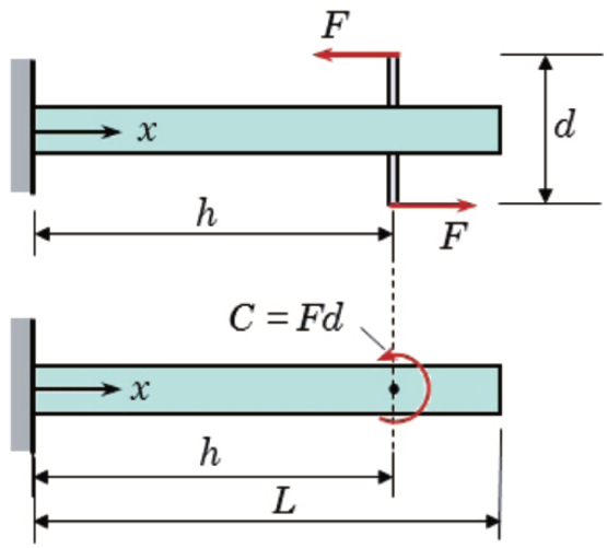
Fig. 6.10 Concentrated couple of two point forces.#
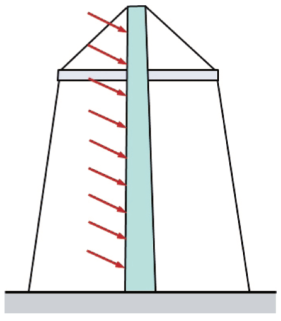
Fig. 6.11 Guyed mast under lateral couples (wind) loading.#
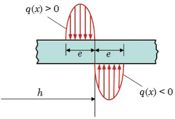
Fig. 6.12 Concentrated couple of nonuniform distributed loading.#
Now we introduce the concept of the internal forces and moments in the beam. For that, we make a virtual cut at an arbitrary position in the beam. In order for the two parts to be in equilibrium, we need to introduce forces and moments acting at the cut on both parts. The forces and moments on the left part are of the same magnitude as the forces and moments on the right part, but have an opposite sign (action is reaction). This is shown in the following figure Fig. 6.13.

Fig. 6.13 Showing the three internal forces and moments.#
In this figure we have three internal forces and moments: the shear force \(V\), the bending moment \(M\) and the normal force \(H\). The positive direction of these forces and moment is according the figure above.
Important
In this course the sign convention for internal forces an moments will be followed by Fig. 6.14.
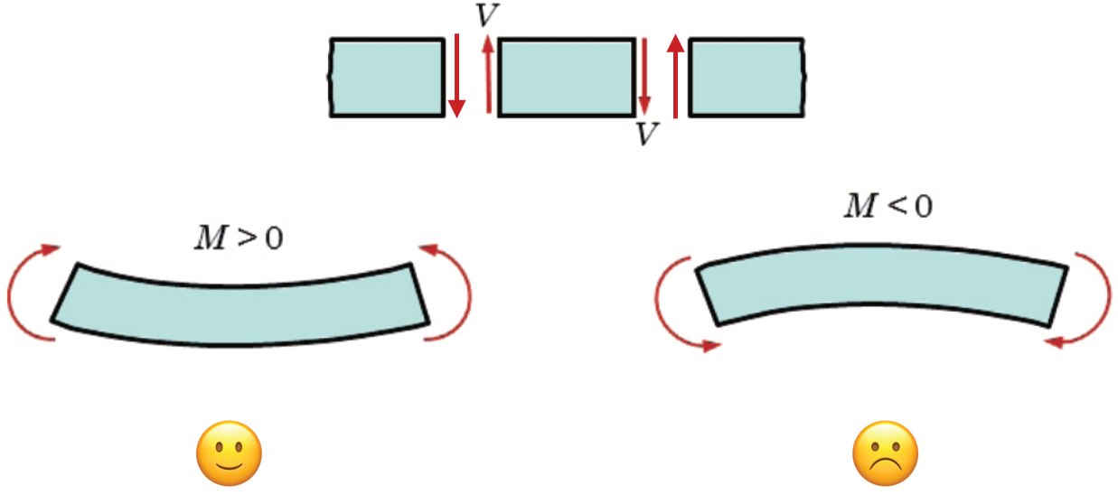
Fig. 6.14 Sign convention of internal forces and moments.#
Note
Other books can use a different convection for the signs of the internal forces and moments.
For statically determinate beams, the internal forces and moments can be determined by applying the equilibrium equations on a part of the beam (see pages 203-204 and the Examples 5.1-5.3).
6.2. Relations between the distributed forces, the shear force and the bending moment#
Force equilibrium in vertical direction for an small piece \(\Delta x\) of a beam experiencing a non-uniformly distributed lateral force \(q(x)\) (Figure 4.24), leads to
If \(\Delta x \rightarrow 0 \), then the following differential equation (DE) is obtained:
Considering the equilibrium of moments around the point Q (Figure 4.24), gives:
Again if \(\Delta x \rightarrow 0, \) the following DE is obtained:
From the first DE, the shear force \(V(x)\) can be obtained by integration on an interval that does not contain concentrated lateral forces (see Figure 5.25):
or the increase in shear force is equal to minus the area under the curve \(q(x)\). Similarly, from the second DE, the bending moment \(M(x)\) can be obtained by integration on an interval that does not contain concentrated couples (see Figure 5.25):
or the increase in bending moment is equal to the area under the curve \(V(x)\).
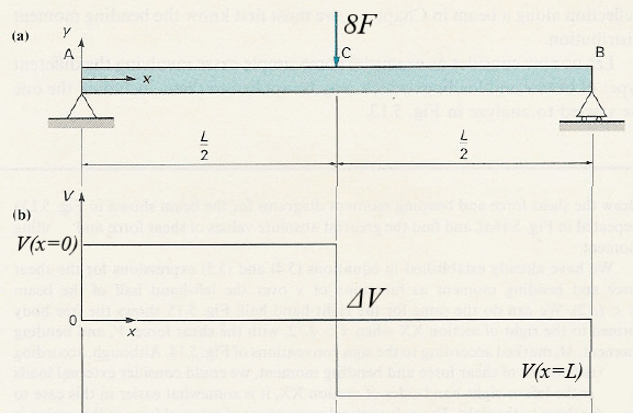
For a concentrated lateral external force \(F\) (positive direction according to fig. 5.14b), we have
where \(\Delta V=V^+-V^-\) and \(\Delta M=M^+-M^-\) with the - and + subscript denoting “just left” and “just right” of the concentrated force, respectively. For a concentrated external couple \(C\) (positive direction according to Figures 5.31 and 5.32), we have
where the \(\Delta V\) and \(\Delta M\) are taken at the position of the concentrated external couple.
The “boxed” equations can now be used to determine and draw the shear force and bending moment diagrams for statically determinate beams. The “fast” procedure will be illustrated with examples during the lectures. Some notes:
Determine reaction forces/moments as a first step.
Take reaction forces/moments into account as known concentrated external forces and couples.
Start with the shear force diagram.
At concentrated external forces there is a “jump” in the shear force curve.
In between the concentrated external forces use the differential expression or integral expression to find \(V(x)\). For \(q(x)=0\), \(V(x)\) is a constant. For \(q(x)=q_0\), \(V(x)\) is linear with slope \(-q_0\).
At concentrated external forces there is a “jump” in the slope of \(M(x)\).
At concentrated external couples there is a “jump” in \(M(x)\).
In between the concentrated external forces and/or external couples use the differential expression or integral expression to find \(M(x)\) from \(V(x)\). For \(V(x)\) is constant, \(M\) is linear. For \(V(x)\) is linear, \(M(x)\) is quadratic. At a point where \(d{V}/{dx}=0\), there is an extremum (maximum or minimum) in \(M(x)\).
Use the Examples 5.4-5.8 to practise the “fast” procedure. Also take a look at Example 6.1 below.
Shear force and bending moment
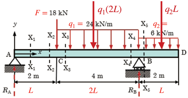
Fig. 6.15 Concentrated couple of nonuniform distributed loading.#
A straight prismatic beam A–D as depicts in Fig. 6.15 has a total length 8 m and is supported at two points.
Straight prismatic beam \(A\)–\(D\): span annotated as \(L+2L+L\) (numerically \(2\ \text{m}+4\ \text{m}+2\ \text{m}=8\ \text{m}\)).
Pinned support at \(A\) (left end): vertical reaction \(R_A\) shown.
Roller support at \(B\), located \(6\ \text{m}\) to the right of \(A\): vertical reaction \(R_B\).
Down-acting point load \(F = 18\ \text{kN}\) applied between the dashed section lines \(X_2\) and \(X_3\).
Uniformly distributed load \(q_1 = 24\ \text{kN/m}\) acts downward over the middle \(2L\) (\(4\ \text{m}\)) segment; its resultant is denoted \(q_1(2L)\).
Uniformly distributed load \(q_2 = 6\ \text{kN/m}\) acts downward over the right-hand \(L\) (\(2\ \text{m}\)) segment; its resultant is denoted \(q_2L\).
Section cuts \(X_1,\;X_2,\;X_3,\;X_4,\;X_5\) are marked along the beam, with \(X_4\) passing through the roller at \(B\) and \(X_5\) to the left of \(D\).
Global axes: \(x\) directed from \(A\) toward \(D\), \(y\) directed upward at \(A\).
Please draw the shear force diagram and the bending moment diagram.
Solution
We start by setting up the equations for a global equilibrium. Thus in equilibrium the vertical equilibrium force and the moment equilibrium about point A are set to zero and we can solve for the reactions \(R_B\) and \(R_A\) through
Now the reaction forces are found to be
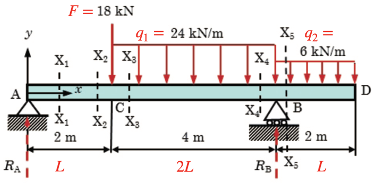
Fig. 6.16 Cleaner depiction of the beam.#
The next step is to make virtual cuts throughout the beam where it is easier to look at the system like in Fig. 6.16 and make virtual cuts like done in Fig. 6.17.
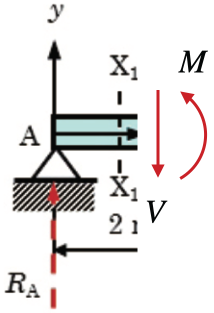
Fig. 6.17 Virtual cut trough the beam.#
Within the segment
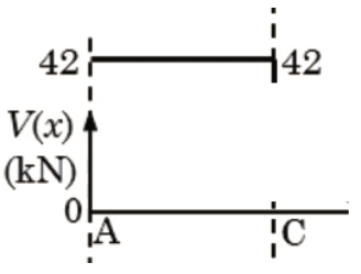
Fig. 6.18 Virtual cut A-C.#
With a virtual cut from A-C (as shown in Fig. 6.18) we get that
With now making following the same procedure throughout the entire beam the shear force diagram and the bending moment diagram can be drawn. The shear force diagram is depicted in Fig. 6.19 below.
The relations \(\displaystyle \frac{d V}{d x} =- q(x), \, \, \Delta V =- F \,\, {\rm and} \, \, V_2-V_1 =- \int_{x_1}^{x_2}q(x)dx\) are used.
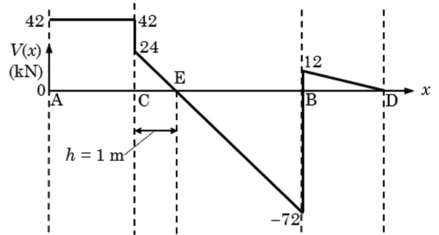
Fig. 6.19 Shear force diagram#
By drawing the bending moment diagram directly below the shear force diagram a clear depiction between the segments of the beam, shear moment and bending moment is established. Thus the final result is given by Fig. 6.20.
Here \(\displaystyle \frac{d M}{d x} =V(x) ,\, \, M_2-M_1 = \int_{x_1}^{x_2}V(x)dx \, \, {\rm and} \, \, \Delta M(x)=-C\) are used.
Fig. 6.20 Shear force diagram#
The computer method described in Section 5.2.3 is not part of the exam
Instead we solve beam problems numerically with the Marc/Mentat finite element package. For the finite element method used in Marc/Mentat (the displacement method) there is no difference in the procedure when solving statically determinate and indeterminate beams.
In each node we have, in addition to the three displacement components (in \(x\), \(y\) and \(z\) direction), three rotations (around the \(x\), \(y\) and \(z\) direction). Furthermore, in each node there are three force and moment components. The members forces and moments can be expressed in the displacements and rotations of the nodes, assuming the members remain connected to the nodes after deformation (compatibility). After substituting these expressions into the equilibrium of forces and moments of all the nodes, a set of equations expressed in the displacements and rotations of the nodes is obtained.
If the kinematic boundary conditions are such that all rigid body modes are suppressed, the system will be regular and can be solved.
Similarly to trusses, the internal forces (shear and normal forces) and moments in the beams can be computed in a post-processing step.