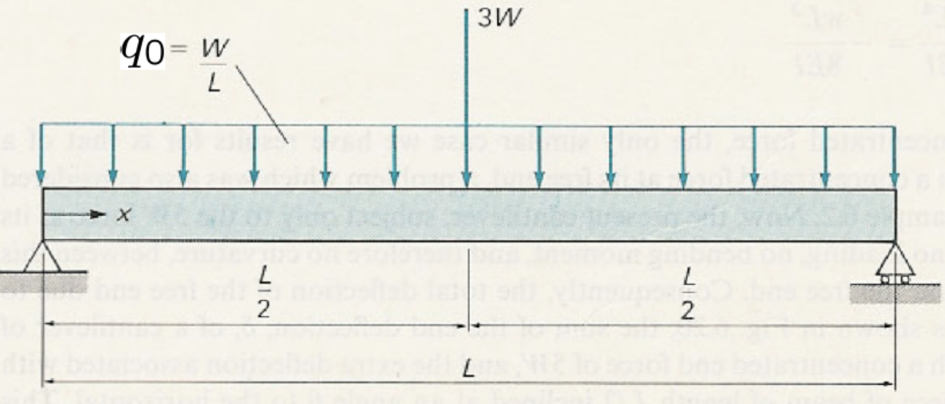

9. Bending of beams: deformation; Application of standard deflection formulas#
Book: Introduction Chapter 6, Sections 6.1 and 6.2 (excluding Subsections 6.2.2 and 6.2.4), Section 6.3 and a replacement for Section 6.4
Consider the displacement of the neutral surface in \(y\)-direction and rotation of the cross-section of the beam as a function of \(x\), as depicted in Fig. 9.1. For statically indeterminate beams, the displacements and rotations are needed for computing the internal forces and moments in the beam. The shear deformation, as depicted in Figure 6.1c, will be neglected. This is allowed for slender beams (see below).
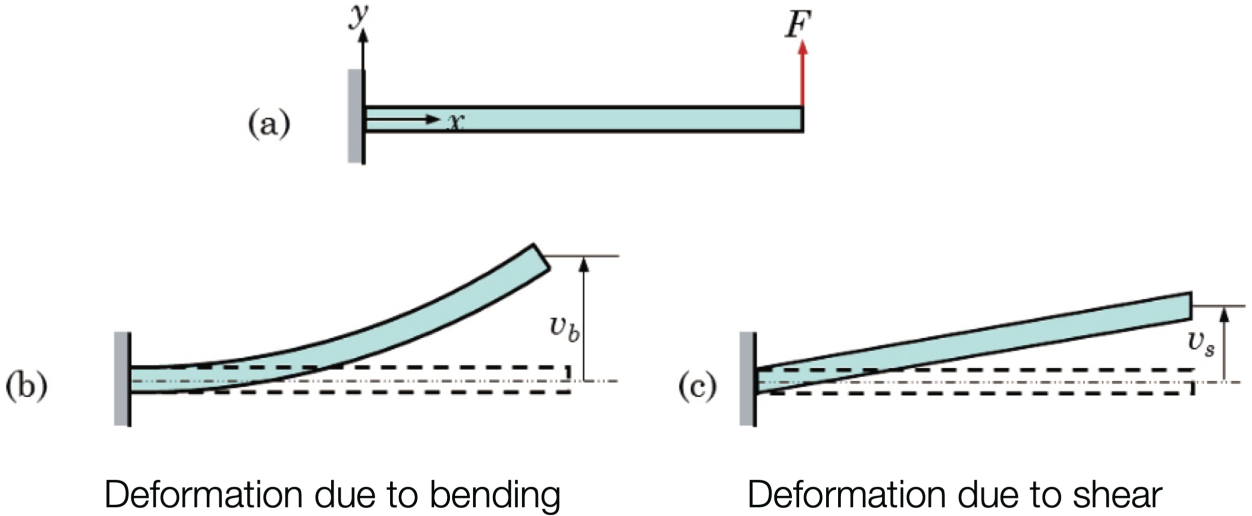
Fig. 9.1 Cantilever deflection: bending yields curved profile; shear yields linear slope. Set criteria of \(\displaystyle v_s \ll v_b\).#
From a previous chapter, we know that:
The product \(EI\) is called the bending stiffness. The lateral displacement of the neutral surface of the beam is denoted by \(v\), which is a function of \(x\). It is assumed that the strains parallel to the cross-section are negligible and that, as an approximation, we can assume that the lateral displacement is the same for all points in the cross-section.
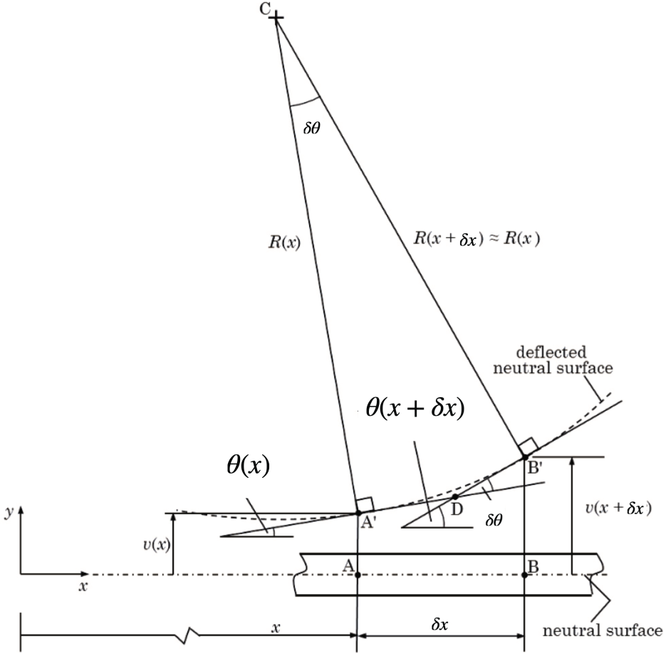
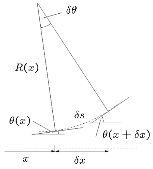
Fig. 9.2 Relation between radius of curvature and lateral displacement \(\nu\).#
Considering Fig. 9.2 above, we see that
but also since the angles are small
which leads to (after equating the two expressions for \(d\theta\)):
Taking the limit \(dx\rightarrow0\), we obtain for small lateral displacement \(v\) approximately:
Substituting this result into the first equations of this chapter gives the important differential equation:
Note, that the positive direction of \(M\) should be defined as in Fig. 6.14.
Because \( {d}M/{{d}x} = V(x) \) and \( {d}V/{d}x = - q(x) \), we find for constant \(I\):
Integration of one of these three differential equations and taking the correct boundary conditions into account, will lead to a solution for the lateral displacement \(v(x)\). The first one is the most easy to use, especially for statically determinate beams. An example for pure bending is given in Example 9.1.
Pure bending
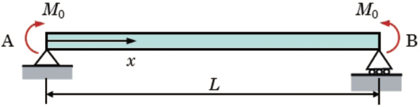
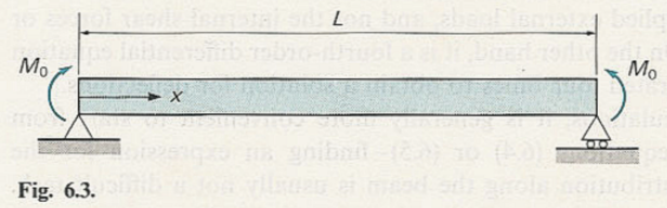
Fig. 9.3 Simply supported beam with equal end moments, constant bending moment.#
The system described in Fig. 9.3 has a prismatic beam of total length \(L\), simply supported at points \(A\) and \(B\) by idealized pinned supports. At each end an equal concentrated moment of magnitude \(M_{0}\) is applied, as shown by the curved arrows at \(A\) and \(B\). A right‐pointing arrow along the beam denotes the positive \(x\)–axis, with the coordinate \(x\) measured from the left support at \(A\) toward the right support at \(B\). The complete loading and support arrangement appear as illustrated. What is the displacement as a function of x along the beam?
Solution
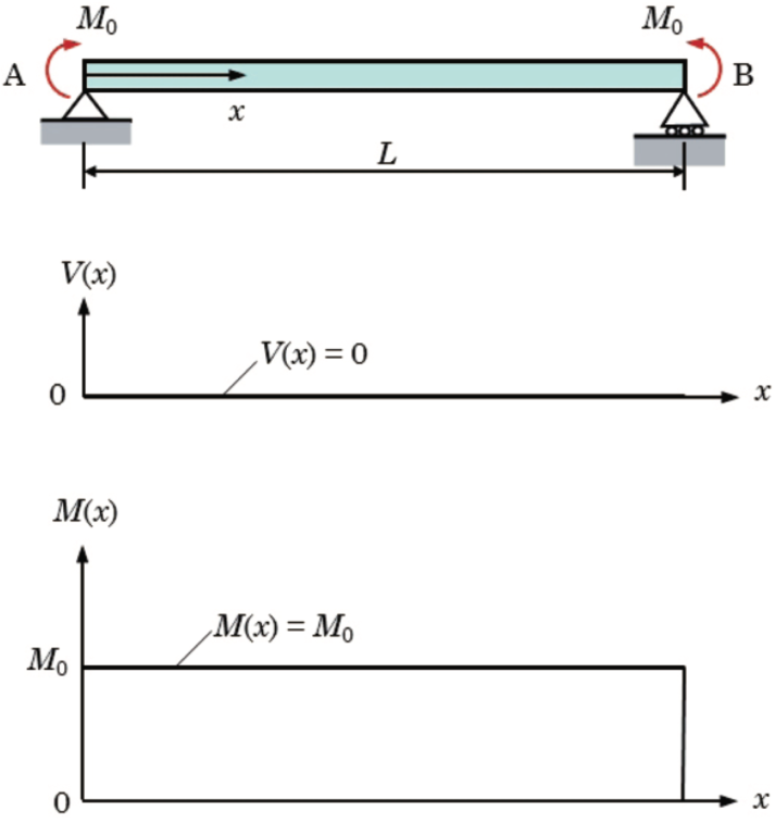
Fig. 9.4 Shear force and bending moment diagrams for the simply supported beam under equal end–moments \((M_{0})\).#
The upper plot in Fig. 9.4 shows the shear force \((V(x))\), which remains exactly zero throughout the span. This reflects the absence of any transverse (vertical) loads on the beam, so there is no change in internal shear from one end to the other. The lower plot in Fig. 9.4 shows the bending moment \((M(x))\), which is a flat line at the level \((M_{0})\) between the supports. This indicates a state of pure bending: the internal moment is uniform and equal to the applied end moments for all \((0<x<L)\), dropping abruptly to zero only at the supports where the beam is free to rotate.
From the moment diagram we find that \( \displaystyle M(x) = M_0 \). With \(\displaystyle M(x) = EI \frac{d^2\upsilon}{dx^2}\) we then find that
Now with integration we find
where \(A\) and \(B\) and constants of integrations that need to be found. This is done by using the boundary conditions \(\displaystyle \upsilon(0)= 0, \ \ \ \upsilon(L) = 0\). Thus \(\displaystyle \implies B = 0\) and \(\displaystyle A = -\frac{1}{2}M_0L\). With thus
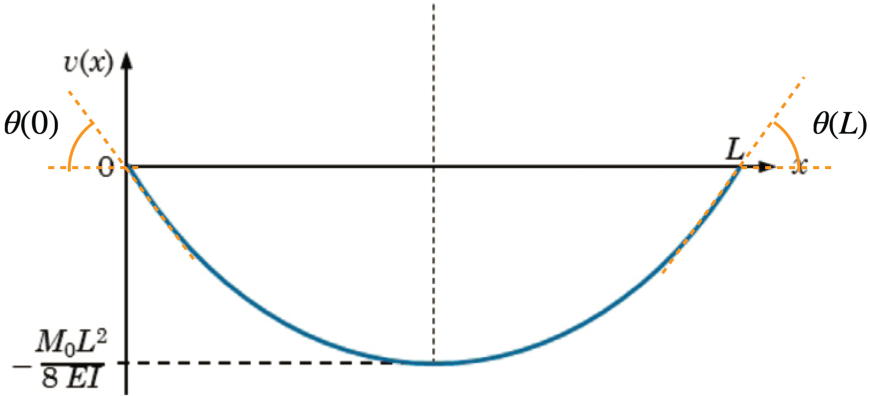
Fig. 9.5 Deflection diagram for beam under pure end–moments \(M_{0}\).#
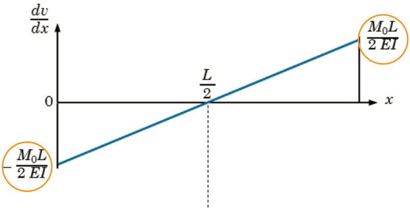
Fig. 9.6 Rotation diagram for beam under pure end–moments \(M_{0}\).#
For the angles and finding \(v_{\min}\) we make a deflection and rotation diagram as shown in Fig. 9.5 and Fig. 9.6. The upper sketch Fig. 9.5 shows the transverse deflected shape \(v(x)\) of the beam, which sags symmetrically under the constant bending moment. The maximum downward deflection occurs at midspan, where
and tangent lines at the ends illustrate the end-rotations \(\theta(0)\) and \(\theta(L)\).
The lower plot Fig. 9.6 is the slope diagram, plotting
against \(x\). It varies linearly from
at the left support, through zero at mid-span, to
at the right support, reflecting the uniform bending moment throughout the span. We can finally do a units check:
Concentrated force
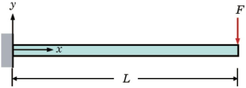
Fig. 9.7 prismatic beam cantilevered from a rigid vertical support.#
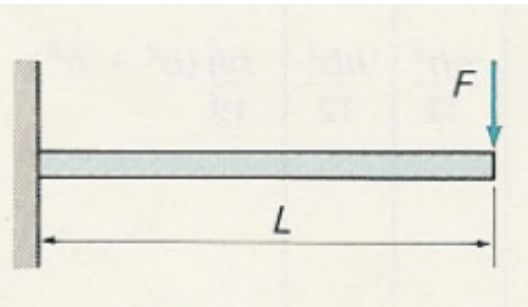
Consider a homogeneous prismatic beam shown in Fig. 9.7 of length \(L\) cantilevered from a rigid vertical support at its left end. A Cartesian coordinate system is shown with the \(x\)–axis directed along the beam from the wall toward the free tip and the \(y\)–axis vertical and upward at the support. At the free end (\(x=L\)) a concentrated transverse load \(F\) acts downward. The support condition, coordinate axes, beam geometry, and end‐load are illustrated as shown. What is the displacement as a function of x along the beam?
Solution
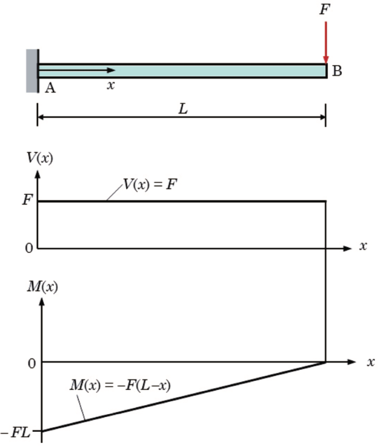
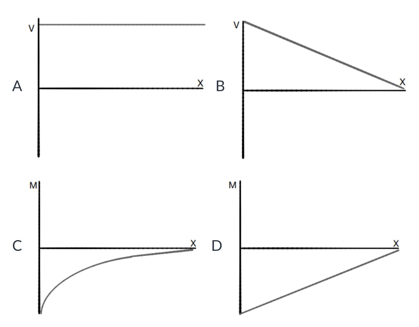
Fig. 9.8 Shear force and bending moment diagrams for the cantilevered prismatic beam.#
From the Moment diagram in Fig. 9.8 we find that \(\displaystyle M(x) = -F(L-x)\), with \(\displaystyle M(x) = EI \frac{d^2\upsilon}{dx^2}\) thus
Integrating twice gives
where \(A\) and \(B\) are integration constants that we find by invoking the boundary conditions \(\displaystyle \frac{d\upsilon}{dx}(0)= 0 , \ \ \ \upsilon(0)= 0\). From here it thus is found that \(\displaystyle \implies A= B = 0\). We can now write
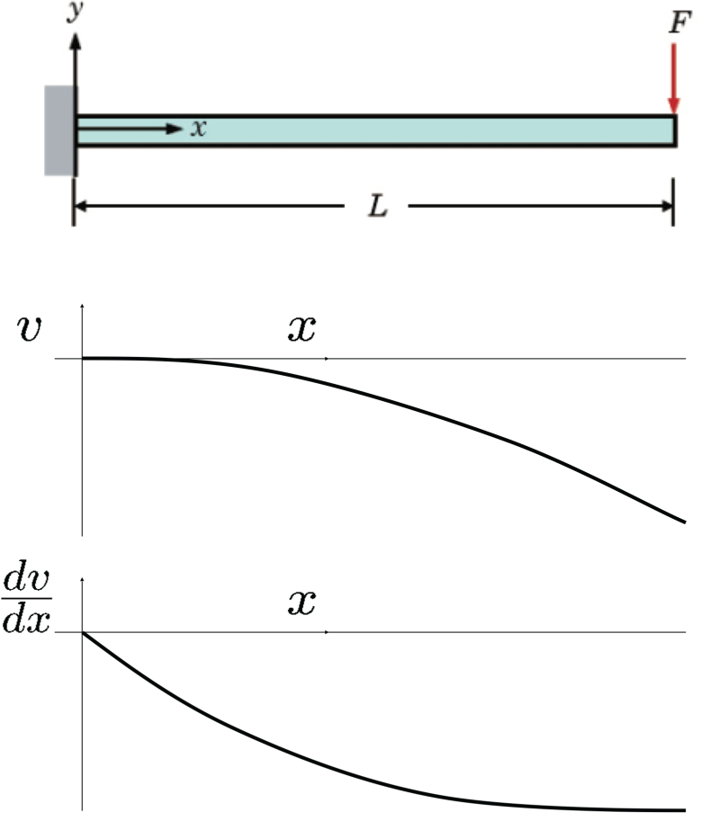
Fig. 9.9 \(\upsilon\) and \(\frac{d\upsilon}{dx}\) plotted with respect to \(x\) for the cantilevered prismatic beam.#
On the right side the deflection curve we have
which is the vertical displacement (downward deflection) of the free end at \(x=L\) under the tip load \(F\). On the right of the slope curve we have
which is the rotation (slope) of the beam’s neutral axis at the free tip due to the same load.
In Example 9.2 two standard formulas are derived: the displacement and slope at the end of a cantilever beam of length \(L\) with a concentrated force \(F\) applied at the free end (see Figure 6.6):
An approximation of the shear displacement \(v_\text{s}\) of a cantilever beam with concentrated force can be obtained as follows. First, assume a constant shear stress distribution on a rectangular cross-section of width \(b\) and height \(d\), i.e. \(\tau=F/{bd}\). The shear displacement now becomes approximately (see Figure 6.1c):
The bending displacement for this case is given by
Assuming \(\nu=0\), the ratio of shear displacement to bending displacement is
which is very small for slender beams (\(d\ll L\)) and the shear deformation can be neglected in that case. The conclusion remains the same for other values of the Poisson ratio.
Distributed load
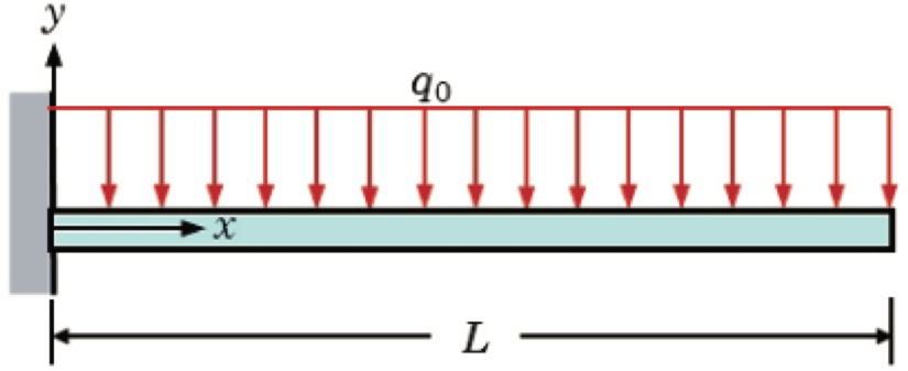
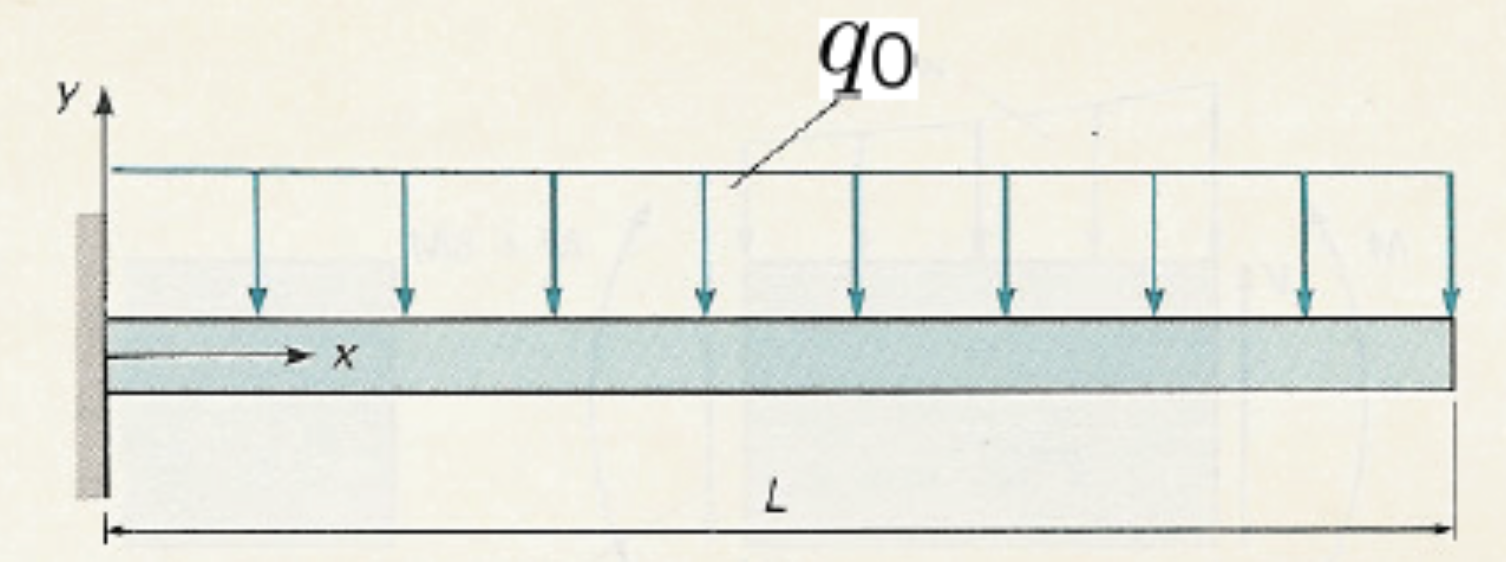
Fig. 9.10 Cantilever beam fixed at the left wall, length \(L\), with the \(x\)-axis running along the beam and the \(y\)-axis upward. A uniform downward distributed load \(q_0\) acts over the entire span, and the right end is free-illustrating the setup for finding the transverse displacement.#
A straight, prismatic cantilever beam \(AB\) of length \(L\) as depicted in Fig. 9.10 is rigidly fixed at the wall at \(x=0\) and free at the tip \(x= L\). The beam has constant flexural rigidity \(EI\) and is loaded along its entire span by a uniform downward distributed load of intensity \(q_0\) (force per unit length).
What is the displacement as a function of \(x\) along the beam?
Solution
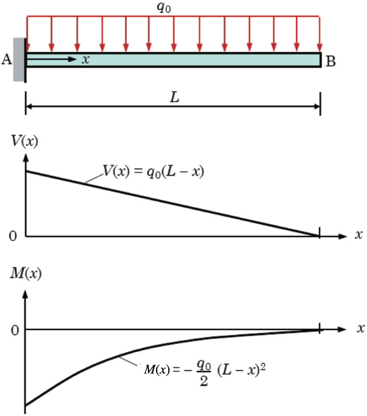
Fig. 9.11 Cantilever beam of length \((L)\) fixed at \((A)\) and free at \((B)\), subjected to a constant distributed load \((q_{0})\). The resulting internal actions are (middle) a linear shear‐force diagram \((V(x)=q_{0}\bigl(L-x\bigr))\) and (bottom) a quadratic bending‐moment diagram \((M(x)=-\dfrac{q_{0}}{2}\bigl(L-x\bigr)^{2})\).#
Cut the beam at a section \((x)\) from the fixed end. By equilibrium of the free‐body to the right of the cut,
Taking moments about the cut gives us
The elastic curve satisfies
Integrate once to get the slope \((v'(x))\):
Apply the boundary condition at the fixed end, \((v'(0)=0)\)
Hence
Integrate again to get \((v(x))\):
Compute the integral:
so
Apply the boundary condition \((v(0)=0)\):
Thus
One may expand and simplify:
At the free tip \((x=L)\),
and
If one replaces the uniform load by an equivalent concentrated force \((\;F = q_0 L)\) acting at the tip, the elementary cantilever tip‐deflection would be \((\;v_{\rm eq} = \tfrac{F L^3}{3EI})\). Comparing,
which correctly recovers our uniformly‐distributed result when \((F=q_0L)\).
In Example 9.3 again two standard formulas are derived: the displacement and slope at the end of a cantilever beam of length \(L\) with a uniform distributed force \(q_0\):
Assignment: derive the two standard formulas for the displacement and slope at the end of cantilever beam of length \(L\) with a concentrated moment \(M\) applied at the free end:
In appendix C several formulas for displacements and slopes for common cases have been tabulated. Also see the Examples 6.4 and 6.5 for a general approach in deriving these formulas.
In Section 6.2.2 it is explained that discontinuities in the shear force and bending moment requires much more effort in finding analytical solutions for the differential equations. The reason is that the regions separated by the discontinuities have different integration constants that need be determined by matching the solutions at the discontinuities. In order to handle these solutions more easily, so-called singularity functions or step functions are introduced. Since we can deal with these complicated cases using a numerical program, such as Marc/Mentat, the step function approach (Section 6.2.2) will not be part of the exam. Moreover, by cleverly using the examples from Appendix C together with superposition, fictitious fixed ends, symmetry conditions and rigid rotation deflection (Dutch: `kwispeleffect’) we can solve beam deflection problems in an alternative way without using the step function approach.
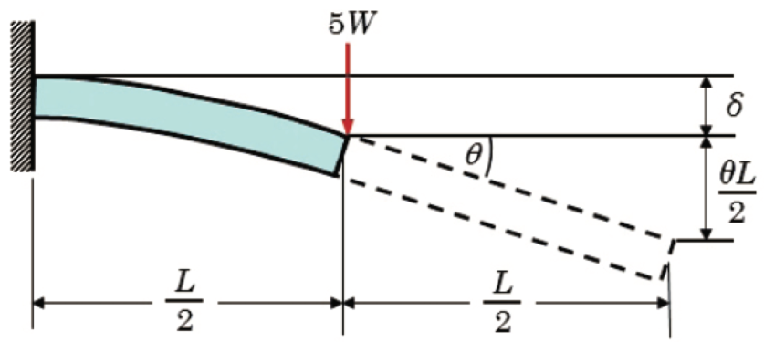
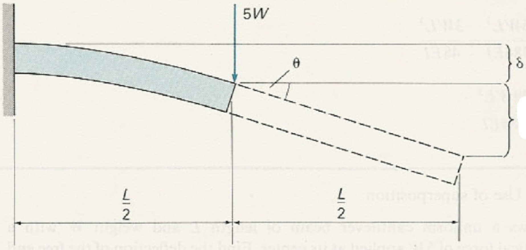
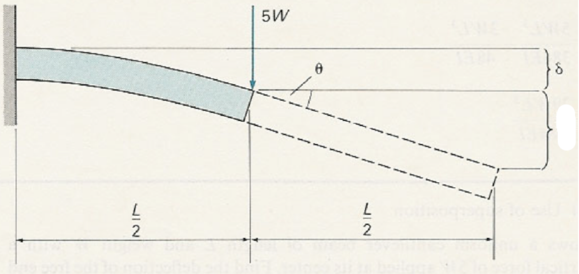
Fig. 9.12 Cantilever beam of total length \((L)\), fixed at the left end, with a concentrated load of magnitude 5 \(W\) applied at its midpoint \(((x=L/2))\). The load causes a downward deflection \((\delta)\) at the point of application and a rotation by angle \((\theta)\); the remaining half‐length then produces an additional vertical displacement of \((\theta,L/2)\) at the free tip.#
If the material behaviour is linear elastic the load can be split into partial loads and the displacements and rotations can be determined by superposition of the results of the partial loads. Examples 6.9 and 6.10 show this procedure. Example 6.10 also shows the application of rigid rotation deflection (Dutch: “kwispeleffect”). For the end displacement of the partial load of the concentrated force (see {numref}’L9-fig12’), we get
The second term is the result of rigid rotation deflection. The solution of this example after superposition of all partial loads (concentrated force and distributed load) is:
Check that the result has the correct dimension of length.
Check the dimension of all (partial) results of deflections and slopes!
Section 6.2.4 on beams of varying cross-section is not part of the exam. However, realise that if the cross-section depends on the axial coordinate \(x\), and thus \(I = I(x)\), the curvature-moment relation becomes more difficult (see Eq. (6.52)). As a result, the integration process of obtaining the deflection \(v(x)\) is more difficult as well. This is shown in Example 6.11.
For simply supported beams it is often possible to use a fictitious fixed end, if we know where the slope is zero. For example for symmetric beams with a symmetric loading the fictitious fixed end can be assumed half way. Now we can apply the standard case of Appendix C for a cantilever to half of the beam using the reaction force and the applied loads to half of the beam. Don’t forget to substitute half the length of the beam in the deflection formulas! Apply this procedure to Example 6.9 and compare with the result in the book.
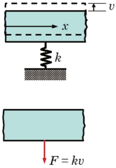
Fig. 9.13 Translational spring model: a rigid block undergoes a linear displacement \(v\) against a spring of stiffness \(k\) with \(F = k\,v\).#
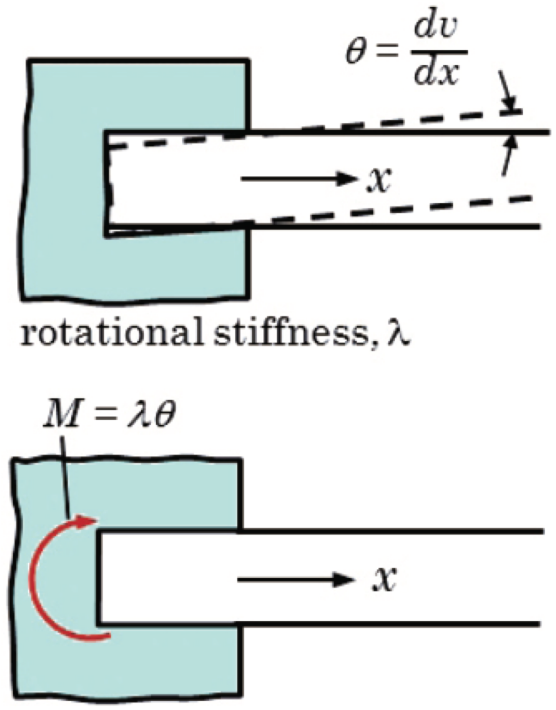
Fig. 9.14 Rotational spring model: a shaft embedded in a housing deflects by a small angle \(\theta=\dfrac{dv}{dx}\) under rotational stiffness \(\lambda\) with \(M = \lambda\,\theta \;=\; \lambda\,\frac{dv}{dx}\).#
9.1. Deflection of statically indeterminate beams#
All examples in Section 6.3 can be solved using the principal of superposition instead of the unnecessary complicated step function approach. For more complicated loading conditions we resort to numerical software.
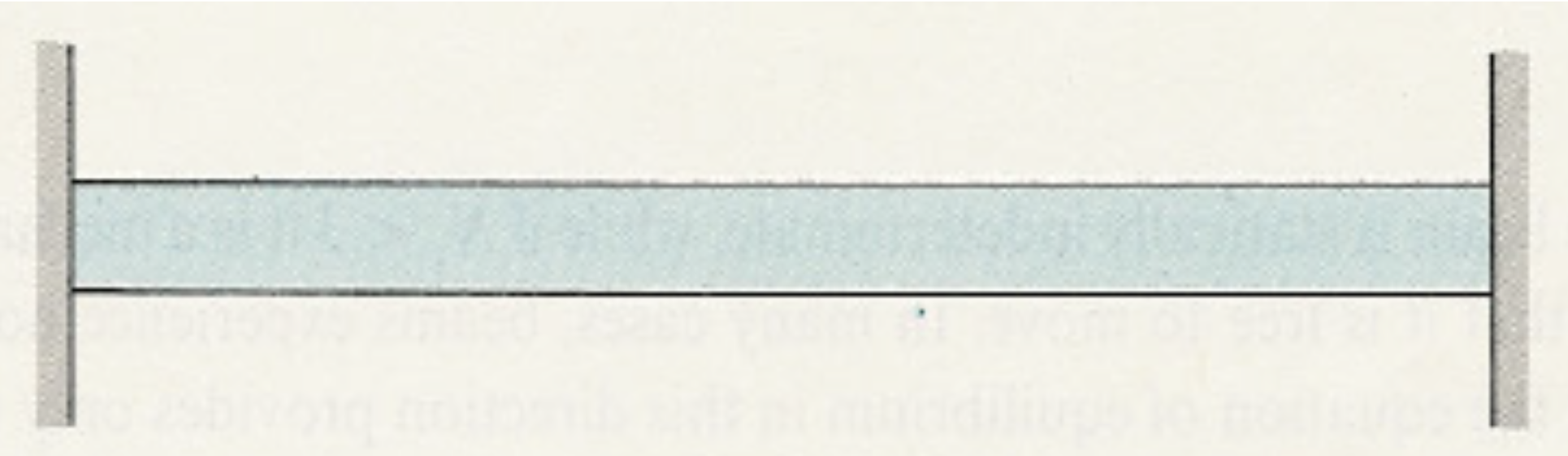
If the number of reaction forces is greater than three, equilibrium alone is not sufficient to determine the forces. In that case, we call the beam to be statically indeterminate. In order for the forces to be determined we need the material behaviour as well.
In Section 6.3 flexible supports are considered. The reaction force in such support is proportional to the deflection or rotation at the support. The ratio of reaction force \(F\) and deflection \(v\) is called the stiffness \(k\) of the support: \(F=kv\). Note, that \(k\) is a positive constant and the directions of \(F\) and \(v\) should reflect that. Similarly, the ratio of reaction moment \(M\) and rotation of the support \(\theta\) is called the rotational stiffness \(\lambda\) of the support: \(M=\lambda\theta\) (see Figures Fig. 9.13 and Fig. 9.14). Again, the rotational stiffness \(\lambda\) is a positive constant.
Solving statically indeterminate beams is not very different from statically determinate beams. First, it is determined which supports are redundant, i.e. not needed to support the beam as a statically determinate one. These supports are replaced by unknown (reaction-) forces and/or moments. Next, the deflections and rotations are computed as a function of the unknown forces and/or moments. Finally, these forces and/or moments are computed by the boundary conditions imposed by the redundant supports. Generally, redundant supports will increase the stiffness of the beam structure.
Examples 6.12 and 6.13 use the step function approach. Instead, these examples should be solved using the standard deflection formulas of Appendix C and the principle of superposition. Try to do this as an exercise and compare the results with the results in the book. In the lectures more details on solving Examples 6.12 and 6.13 will be given.
Section 6.4 will not be part of the exam. It is replaced by the text below.
Except for a single beam with a simple load, solving more complicated beam structures is a lot of work and doing this by hand is almost impossible. Therefore a systematic and automated computer method is needed: the finite element method. The method doesn’t distinguish statically determinate and indeterminate structures, because the displacements instead of forces are the primary unknowns. Computing forces is a post-processing step.
The finite element method consists of several steps. The first step is a division of the beam structure into small pieces (elements). The elements are connected to each other in the nodes. In these nodes the displacement degrees of freedom (three translations and three rotations for a beam) are defined. The second step is cutting each element from the beam structure at the nodes and introducing forces/moments that act on the element. For standard beam elements the two ends of a straight beam define the nodes. In these nodes the corresponding forces/moments that act on the beam are defined. The third step is computing the stiffness of single elements, i.e. the relation between the displacement degrees and forces/moments on an element. For this step the standard formulas of Appendix C could be used. The fourth step is that equilibrium of forces and moments in the nodes is applied and the relations obtained in the third step are substituted. In that way a system of linear equation for the displacements in the nodes is obtained. After taking the specified forces and displacements into account, this system can be solved. The last step is the post-processing step, in which the forces, moments, bending stresses and strains can be computed from the displacements in the nodes.
The computer program based on the finite element method which we use in this course is Marc/Mentat. Try to solve the Example 6.16 using Marc/Mentat and compare with the results in the book.