
10. Torsion#
Book: Introduction to Chapter 7, Sections 7.1, 7.3 (excluding Example 7.8) and 7.4
The general theory for deformation of a beam due to torsion is quite complicated and will not be a subject in this course. However, for the omnipresent solid and hollow cylindrical beams (shafts), the theory is much simpler and will be part of the exam. Examples of cylindrical beams are given in Figures 7.1 (a car transmission) and 7.2 (torsion of coil springs).
We start with the most easy case.
10.1. Torsion of thin-walled cylinders#
The result of this section can be derived quite easily as a special case of the solid hollow cylinders in Sections 7.1.2 and 7.1.3.
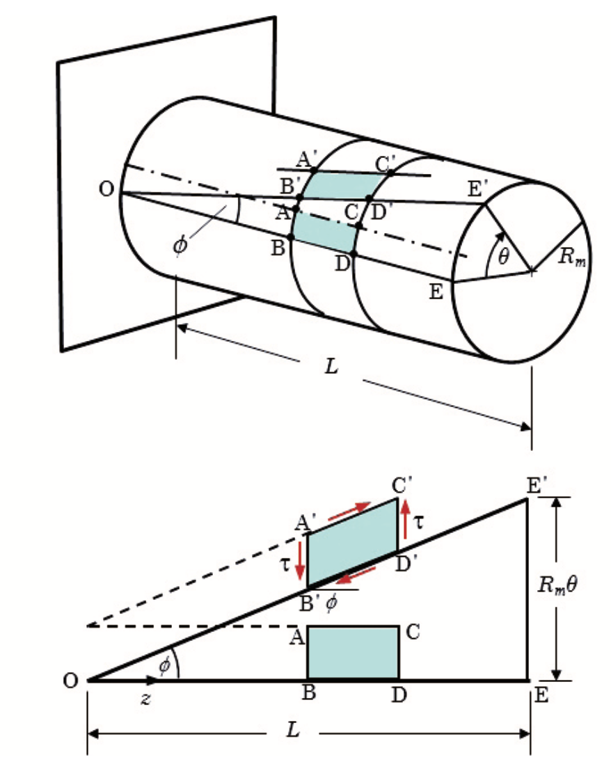
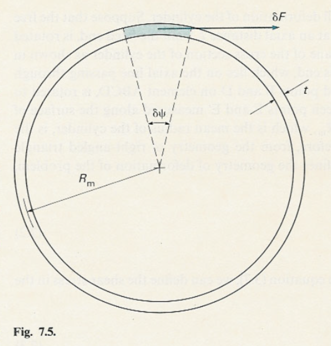
Fig. 10.1 Schematic representation of a thin-walled cylinder of length \(L\) and mean radius \(R_{\textrm{m}}\) subjected to a torque \(T\). The applied torque produces a shear strain \(\phi\) and a relative twist \(\theta\). The lower figure shows the unwrapped cylinder wall, where the shear stress \(\tau\) acts tangentially, and the angular deformation corresponds to \(\theta = \tfrac{TL}{GJ}\) with \(J = 2\pi {R_\text{m}}^3 t \).#
The most important result is: the rotation \(\theta\) of the free end relative to the fixed end of a thin-walled cylinder loaded with a moment (or torque) \(T\) at the free end (see Fig. 10.1) is given by:
Since the rotation is proportional to the length we sometimes write:
Comparing this to the bending formula \(\dfrac1R=\dfrac{M}{EI}\rule[-4mm]{0pt}{4mm}\), we can identify the rotation per unit length \(\dfrac{\theta}L\) as the torsion strain and \(GJ\) as the torsion stiffness.
10.2. Torsion of solid circular shafts#
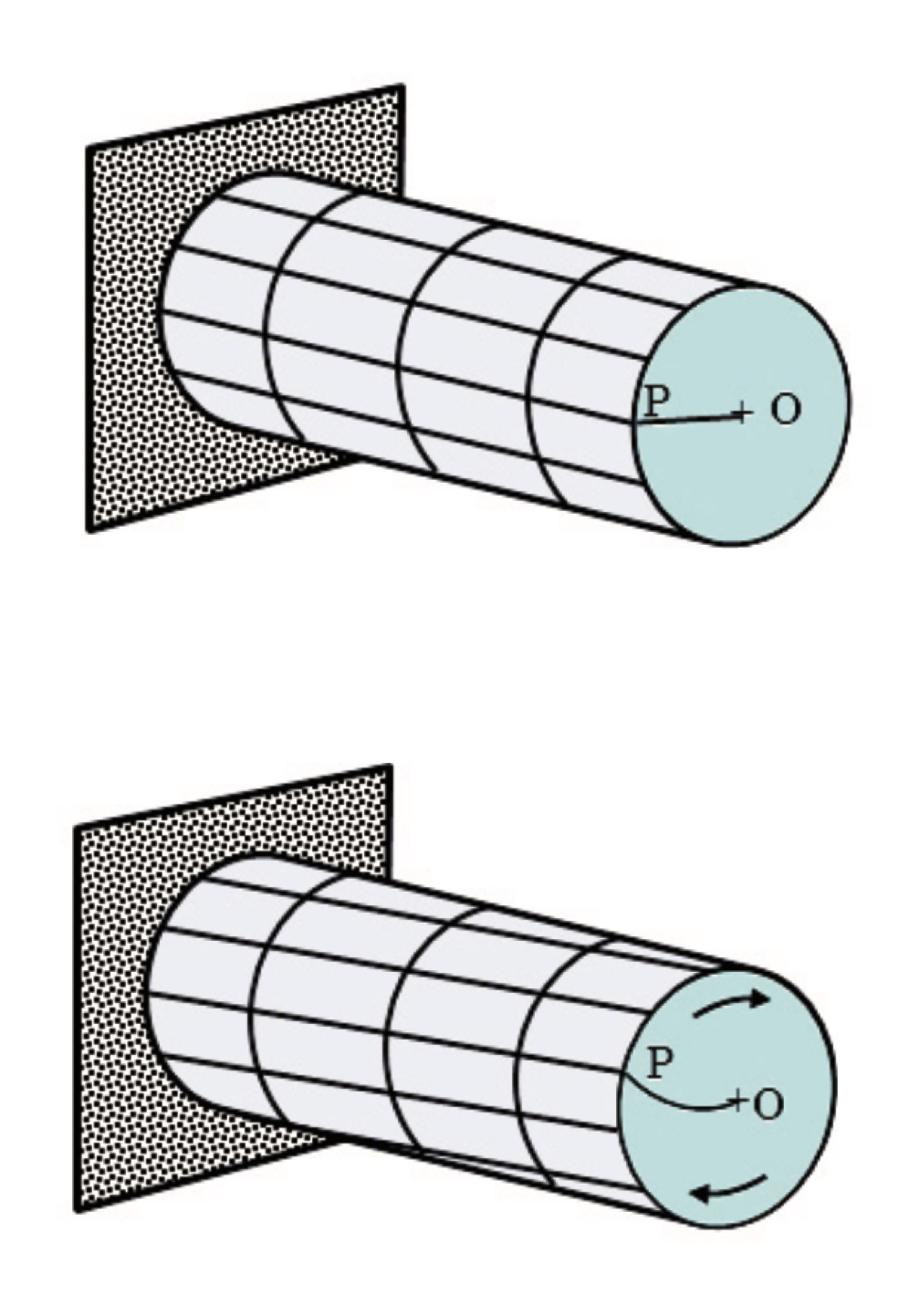
Fig. 10.2 Representation of a solid circular shaft under torsion, modeled as a set of concentric thin-walled cylinders. Each cylindrical layer deforms by shear, producing a uniform twist about the axis \(O\), with shear stress \(\tau\) acting tangentially at a point \(P\) at radius \(r\).#
A solid circular shaft behaves like a set of concentric thin-walled cylinders. See Fig. 10.2. Using symmetry of a small slice of the shaft (see Fig. 10.3), it can be shown that plane cross-sections remain plane and radial straight lines remain straight after applying a torsional load.
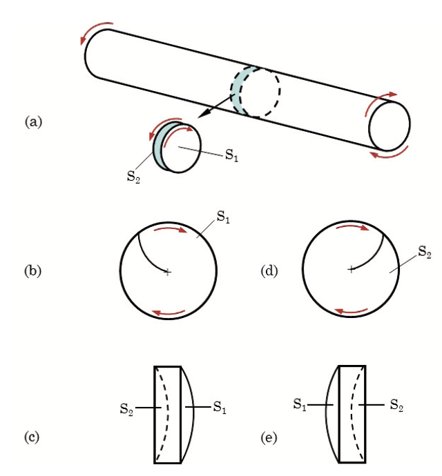
Fig. 10.3 Illustration of warping in a circular shaft under torsion. (a) A shaft element showing surfaces \(S_1\) and \(S_2\). (b–c) Warping displacement of surface \(S_1\), viewed in cross-section and longitudinally. (d–e) Warping displacement of surface \(S_2\), showing compatibility between adjacent surfaces. The deformation preserves cross-sectional circularity while allowing axial warping.#
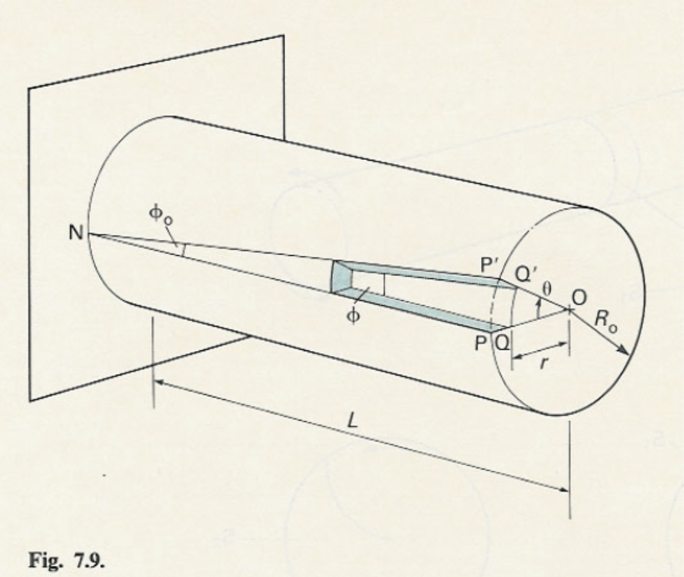
Consider the solid shaft in Figure 7.9. It is fixed on one side and load with torque \(T\) at the other end. On the outer surface we have: \( \text{arc length PP}' = \tan(\phi_\text{o})L = R_\text{o} \theta\), and using the definition of the shear strain \(\gamma_\text{o} = \tan(\phi_\text{o})\), we get \(\gamma_\text{o} = {R_\text{o}\theta}/{L}\). On an imaginary concentric cylinder with radius \(r\) we find analogously \( \gamma (r) = {r \theta}/{L}\). Applying Hooke’s law, the shear stress becomes
The shear stress is a linear function of \(r\) and the maximum value of the shear stress is at the outer surface:
The total torque \(T\) is the sum of the infinitesimal torques \( \delta T=\tau \delta A r\):
Defining the polar second moment of area \(J\) as
we find
The shear stress expression becomes \( \tau (r) = {Tr}/{J} \), which is similar to the expression for the bending stresses: \(\sigma = - {My}/{I}\). For the maximum shear stress at the outer surface we have:
which is again similar to the expression for the maximum bending stress:
10.3. Torsion of hollow circular shafts#
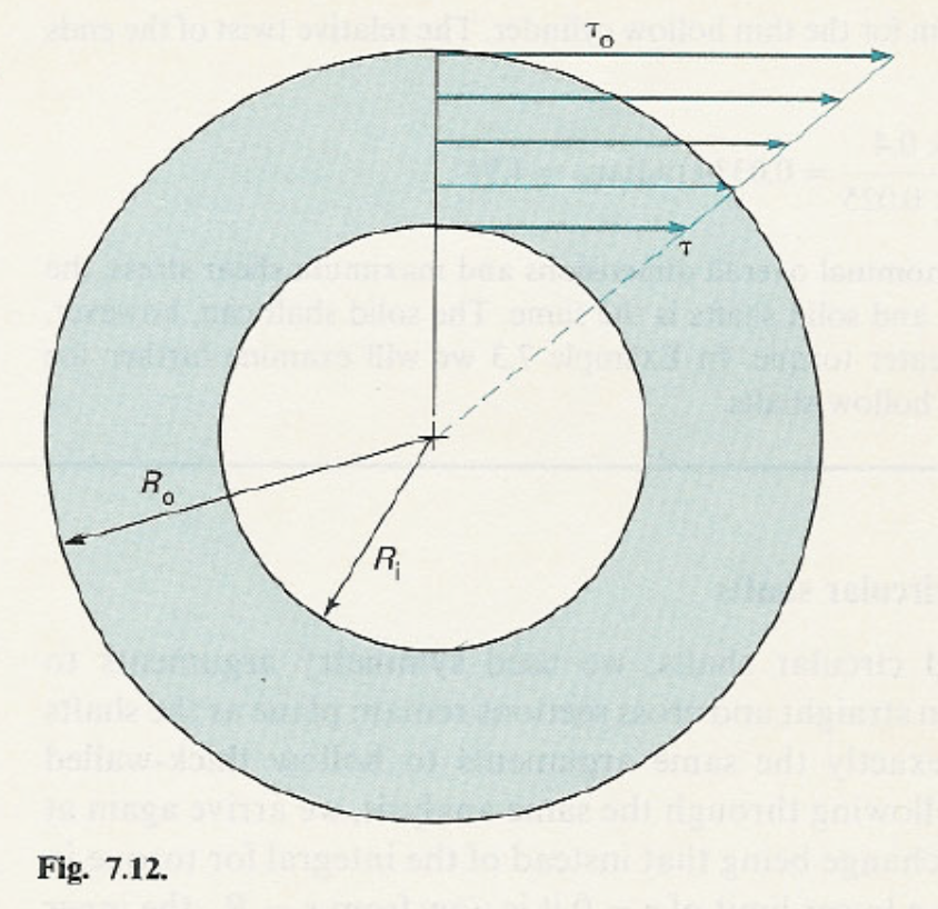
The arguments used for deriving the expressions for a solid circular shaft also apply to a hollow circular shaft. For the polar second moment of area we find for this case:
For a thin-walled cylinder we have \( R_\text{i} \approx R_\text{o} \approx R_\text{m} \) with \(R_\text{m}\) the mean radius. Therefore, we get
For a wall thickness of 20% of the inner diameter, the error in \(J\) for the thin-walled cylinder approximation is \(1.2\%\). The usefulness of the approximate formula is limited, since the exact one isn’t difficult to apply either. However, it does show that for a constant thickness cylinder \(J\) scales with the radius to the power three.
10.4. Nonuniform circular shafts#
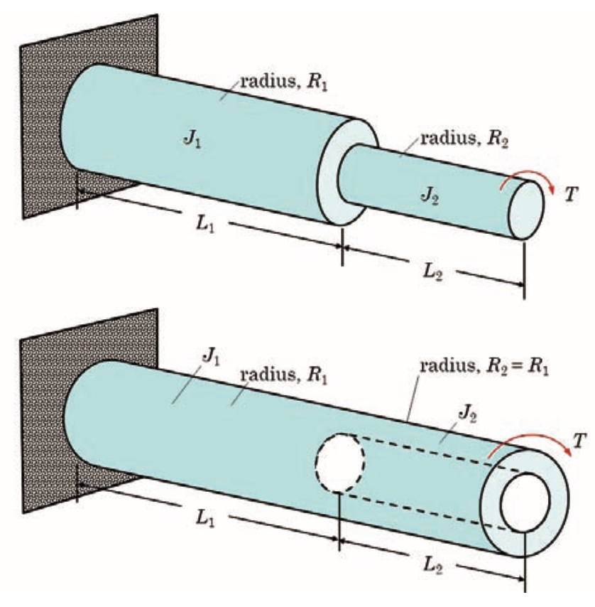
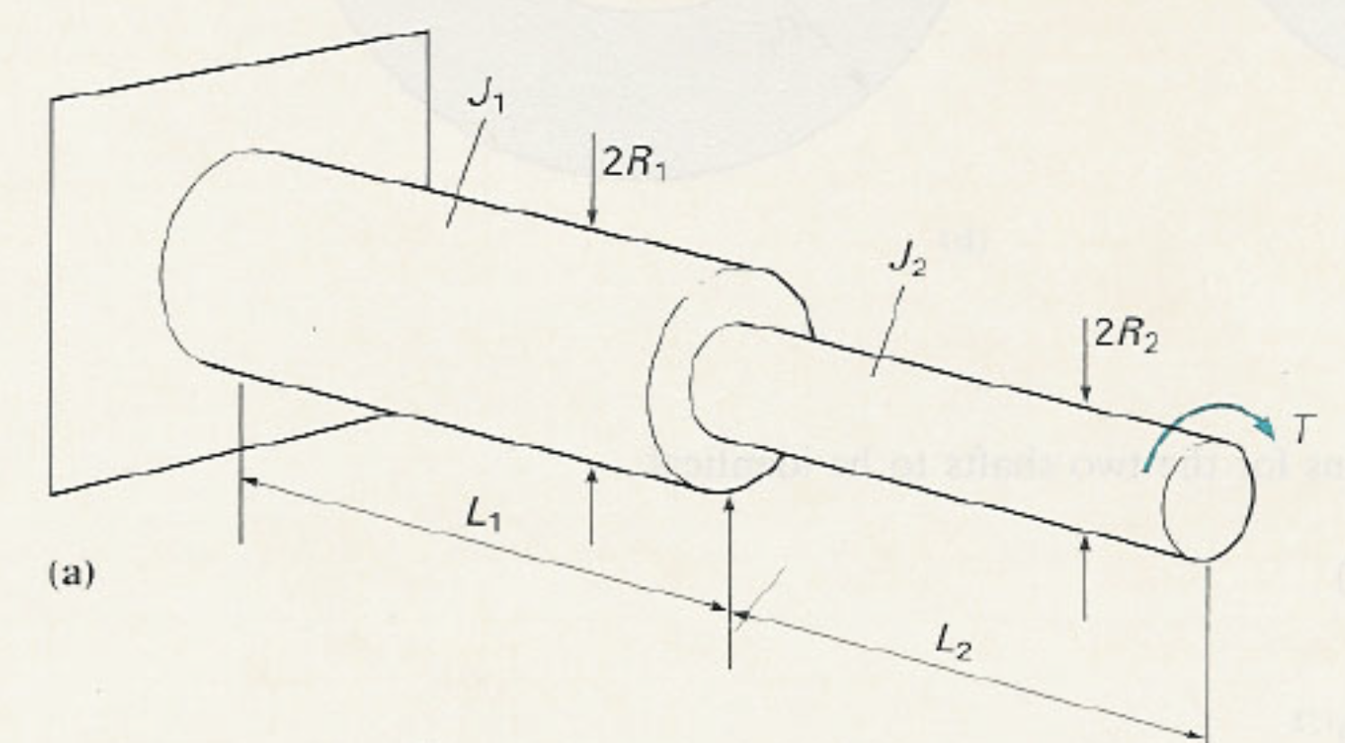
Fig. 10.4 Torsional deformation of composite shafts. The top figure shows two solid shafts of lengths \(L_1\), \(L_2\) and radii \(R_1\), \(R_2\), with polar moments of inertia \(J_1\), \(J_2\), connected in series under an applied torque \(T\). The bottom figure shows a solid shaft of length \(L_1\) and radius \(R_1\) connected to a hollow shaft of length \(L_2\) with inner and outer radii, carrying the same torque \(T\). The twist is distributed according to \(\theta = \tfrac{TL}{GJ}\) for each shaft segment.#
In the examples given in Fig. 10.4, the two parts with lengths \(L_1\) and \(L_2\) have a different value for the polar second moment of area: \(J_1\) and \(J_2\). The rotation of the cross section at the end is the sum of the separate contribution of the two parts:
These examples can be generalised to a continuously varying cross section, where the end rotation is the sum of an infinite number of infinitesimally small contributions:
In the example given in Figure 7.16 we find: \( J(z) = J(0)(1-\alpha z)^4 = J_1 (1-\alpha z)^4 \), which leads to
The maximum shear stress is given by:
which is maximal at the outer surface in the smallest cross section.
If the number of unknown reaction torques is equal to one, the torsion problem is statically determinate, since there is also one equilibrium equation for the torque. This is explained at the beginning of Section 7.2.
Shafts are often used to transmit power, as in the transmission of a car. The power \(P\) is defined as the energy transmitted per unit time and is given by \(P = T\omega\), where \(\omega\) is the rotational speed in radians per unit time. In SI units \(P\) is in Watt, \(T\) in Nm and \(\omega\) in rad/s (or just \(\text{s}^{-1}\)).
The text in Section 7.2 after Example 7.5 about gears is not part of the exam.
If the shaft is statically indeterminate, the solution is found by considering one or more unknown torsion (reaction) moments and an equal number of additional kinematic conditions for the rotation. This is illustrated in the Example 7.7 of Section 7.3. The second example of that section (Example 7.8) can be skipped.
Examples 7.9 and 7.10 of Section 7.4 show displacements and rotations as a result of combined bending and torsion.
Statically indeterminate torsion
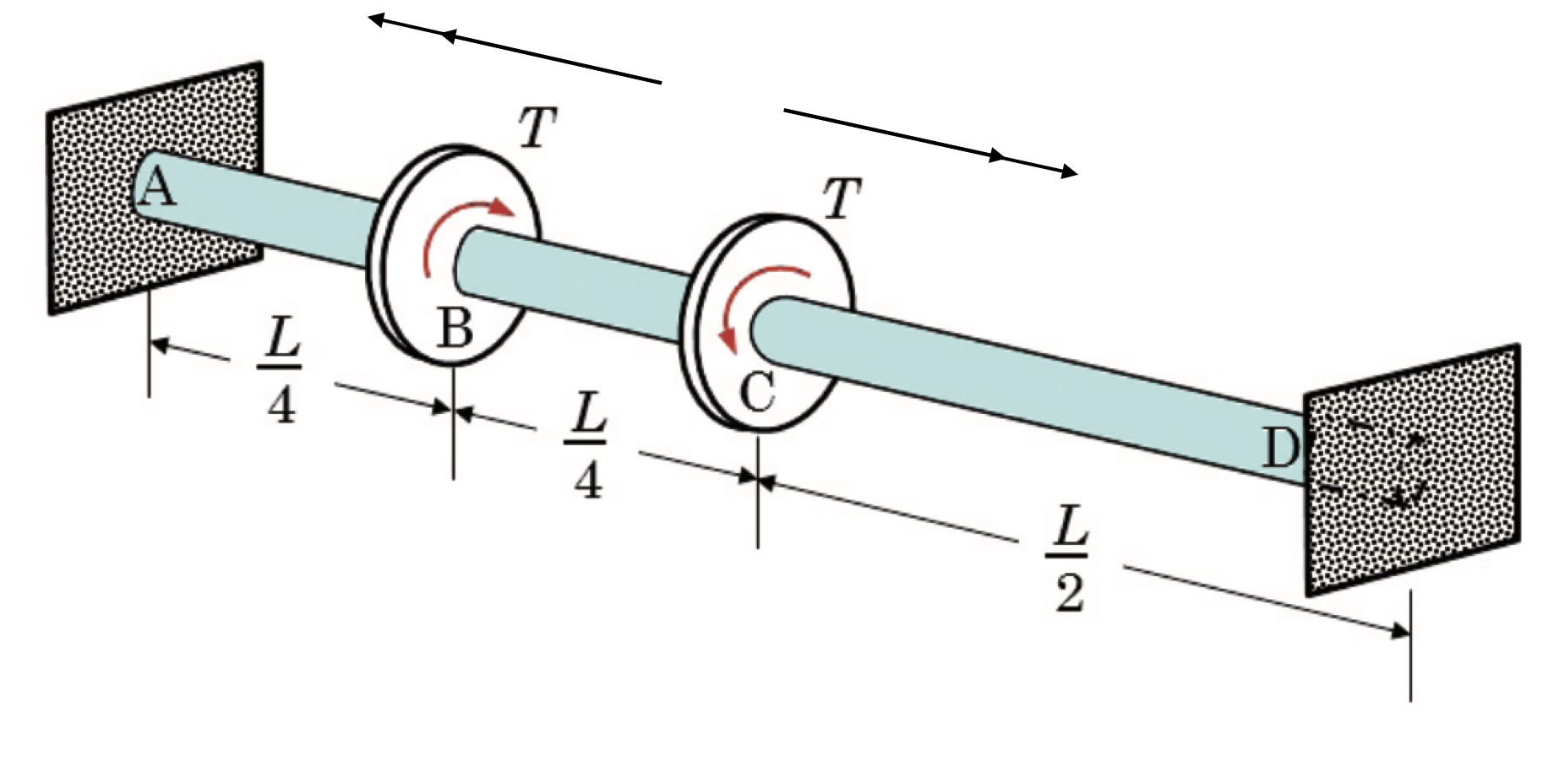
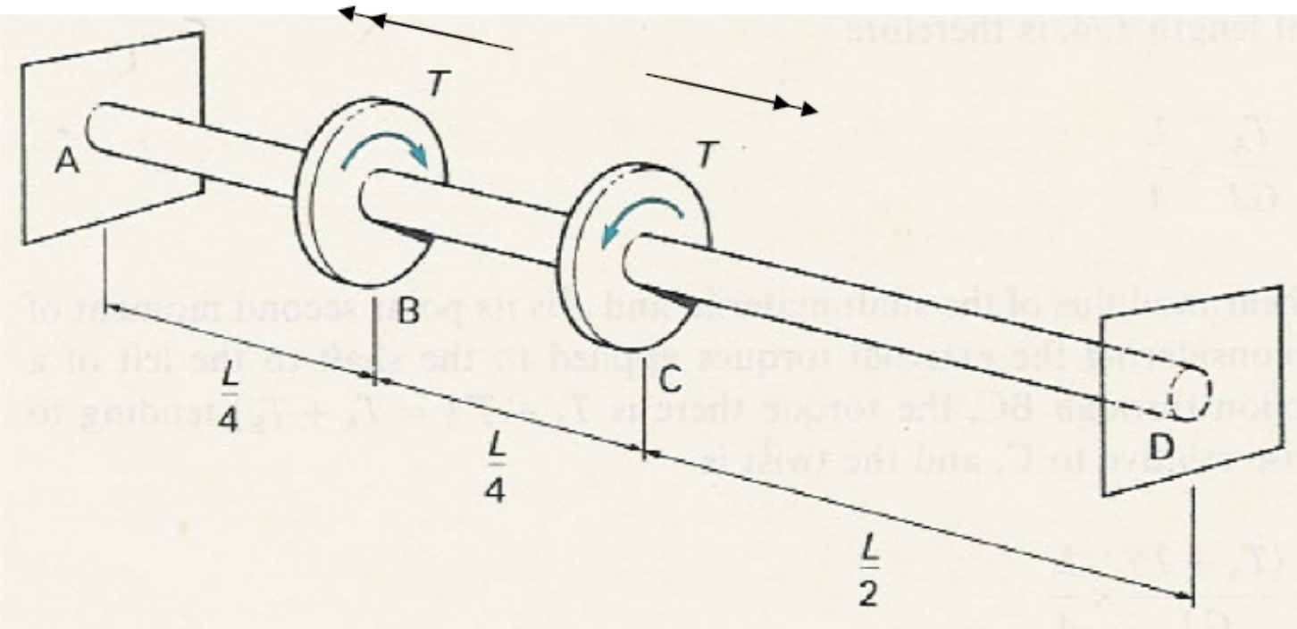
Fig. 10.5 Torsion of a stepped shaft with applied torques. A shaft \(AD\) of total length \(L\) is fixed at both ends. Torques \(T\) are applied at sections \(B\) and \(C\), located at \(L/4\) and \(L/2\) from the supports, respectively. The system illustrates equilibrium of internal torques and compatibility of twist, with angular displacements governed by \(\theta = \tfrac{TL}{GJ}\).#
In this problem we are going to assess the shaft that may be seen in Fig. 10.5. The goal is to find torsion reaction moments at \(A\) and \(D\), \(T(z)\) and \(\theta(z)\). The analysisi of \(T(z)\) should be done through a torsion moment diagram.
Solution
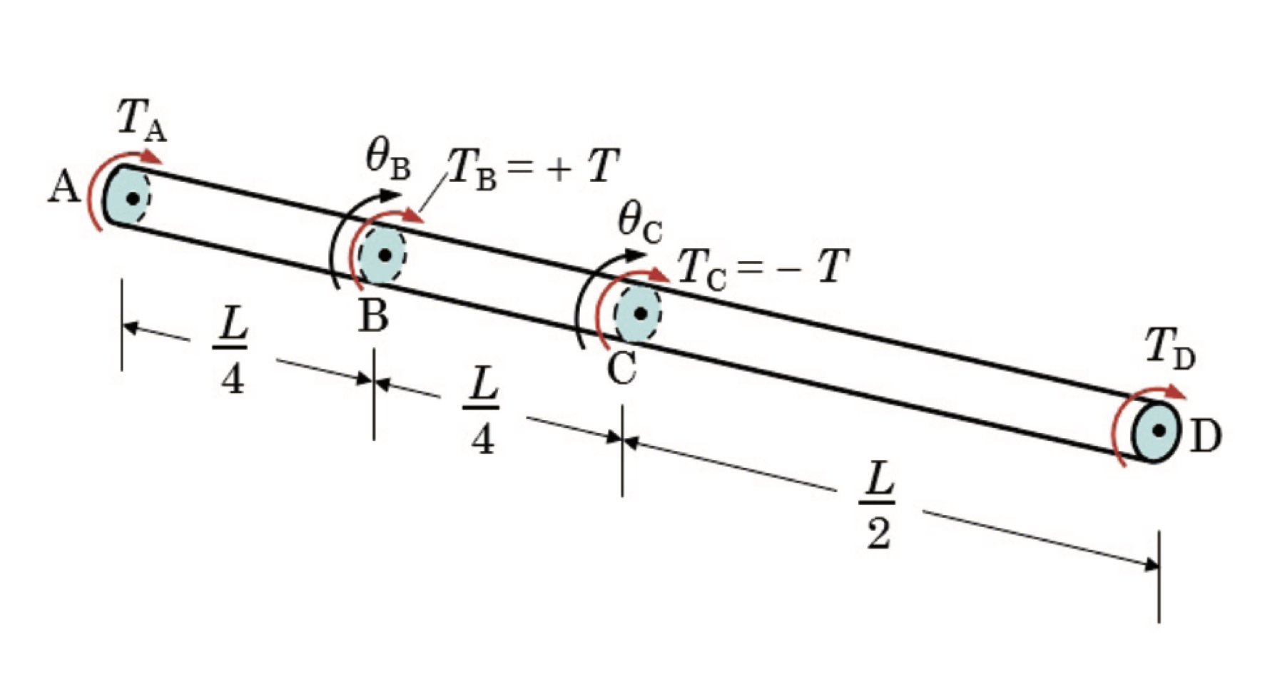
Fig. 10.6 The torsion of the stepped shaft is isalated where a global equilibrium has been applied.#
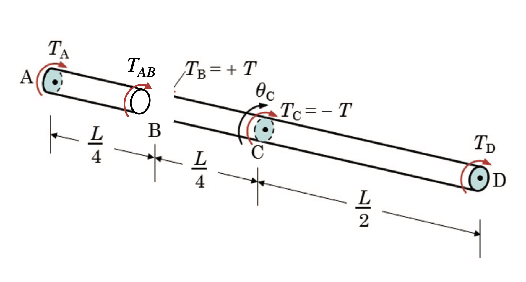
Fig. 10.7 The torsion of the stepped shaft on the analysis of the \(AB\) equilibrium.#
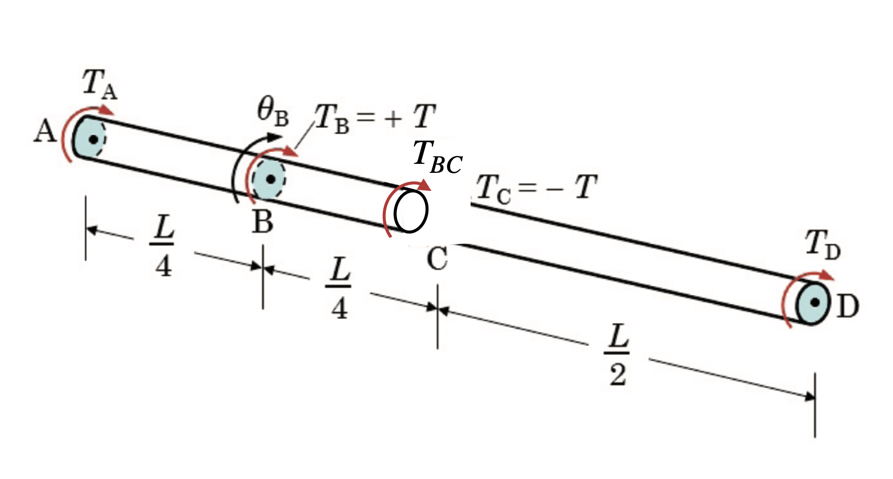
Fig. 10.8 The torsion of the stepped shaft on the analysis of the \(AC\) equilibrium.#
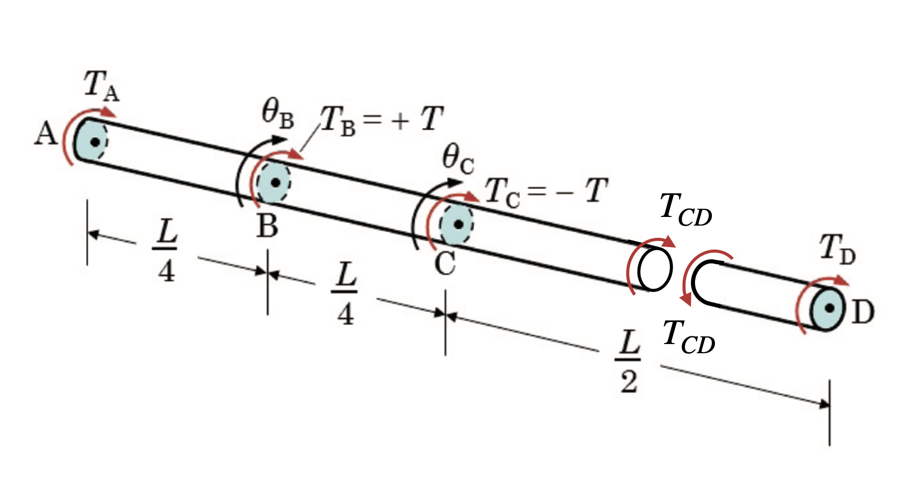
Fig. 10.9 The torsion of the stepped shaft on the analysis of the \(CD\) equilibrium.#
We thus have found that
For the total relative rotation of \(D\) against \(A\)..
With this it can now be shown that \(\displaystyle \implies T_A = -\frac{T}{4}\) and hence \(\displaystyle T_D = \frac{T}{4}\).
Now \(T_{AB}, T_{BC}\) and \(T_{CD}\) can be related to \(T\) by
From here the torsion moment diagram can be restructed which is shown in Fig. 10.10 below.
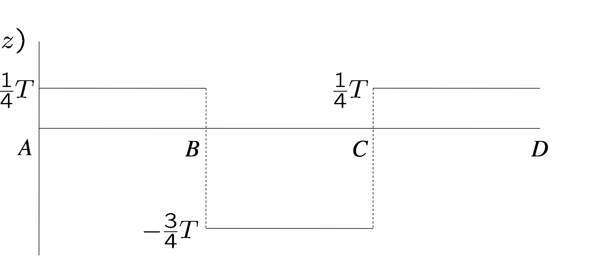
Fig. 10.10 Torsion moment diagram for the stepped shaft.#
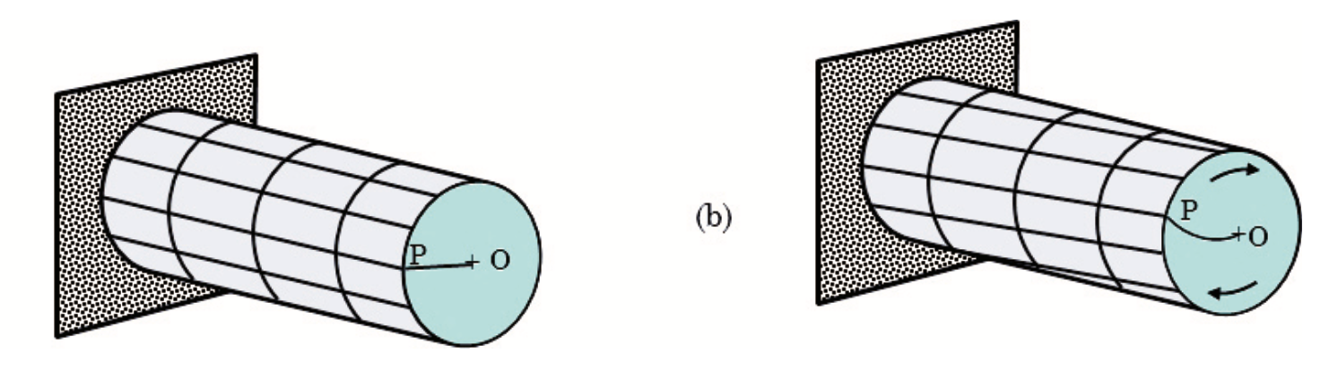
Fig. 10.11 Relative rotation of \(\theta\) with respect to each shaft equilibrium.#
Now for the relative rotation \(\theta(z)\) which may be analysed on basis of Fig. 10.11 by….
From here we may also graph the \(z\) coordinate as a function of the angle \(theta\). This is shown in Fig. 10.12 below.
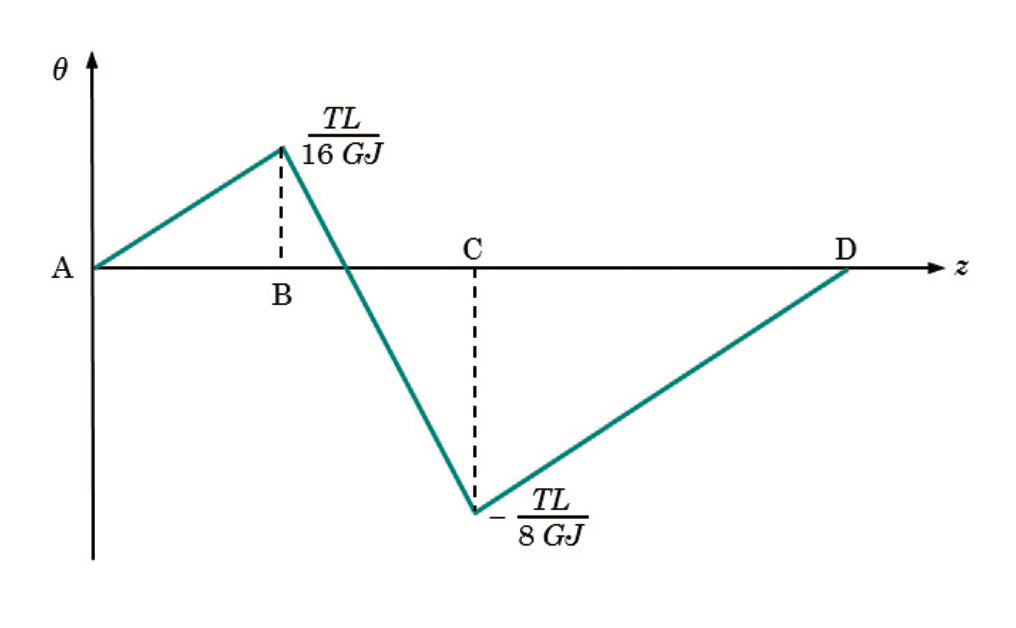
Fig. 10.12 \(z\) as a function of \(\theta\) for the stepped shaft.#
To find the relation between \(T_D\) and \(T\) we set a superposition between \(\theta_D\) and \(\theta_A\) where we get
Below in Fig. 10.13 is a complimentary overview of \(z\) as a function of \(\theta\) for each segment.
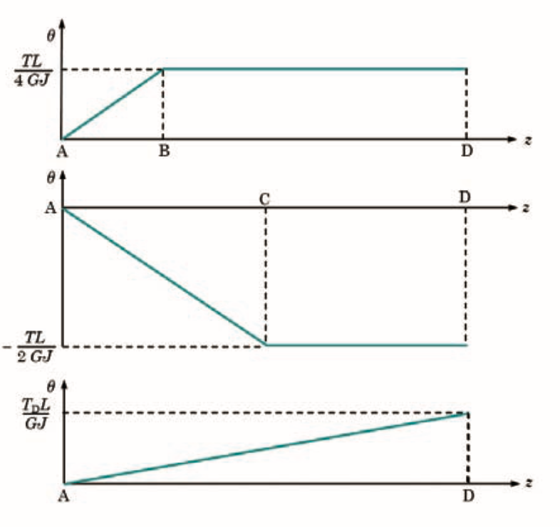
Fig. 10.13 \(z\) as a function of \(\theta\) for the stepped shaft split into each equilibrium segment.#
Combined bending and torsion
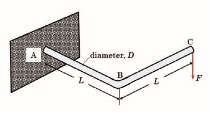
Fig. 10.14 Cantilevered L-shaped circular rod with arms of length \(L\) and diameter \(D\), fixed at \(A\), kink at \(B\), and a vertical tip load \(F\) applied at the free end \(C\); deformation involves coupled bending and torsion of the two legs.#
A L-shaped cantilever may be seen in Fig. 10.14 above. \(E\) and \(\nu\) are known material constants. What is the amount by which \(C\) moves down?
Solution
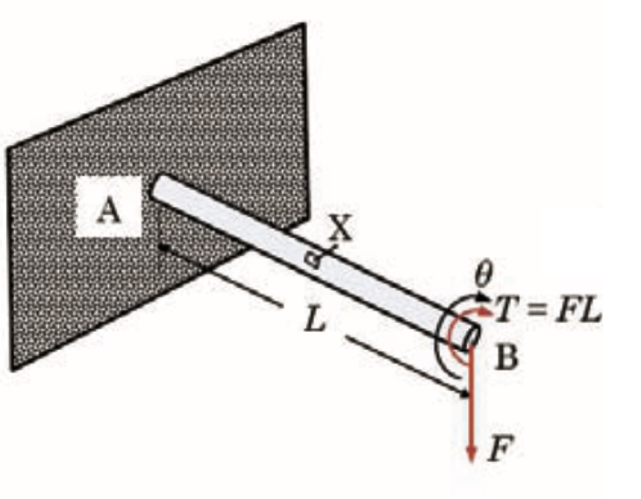
Fig. 10.15 First (left) split off segment from the entire L shaped cantilever.#
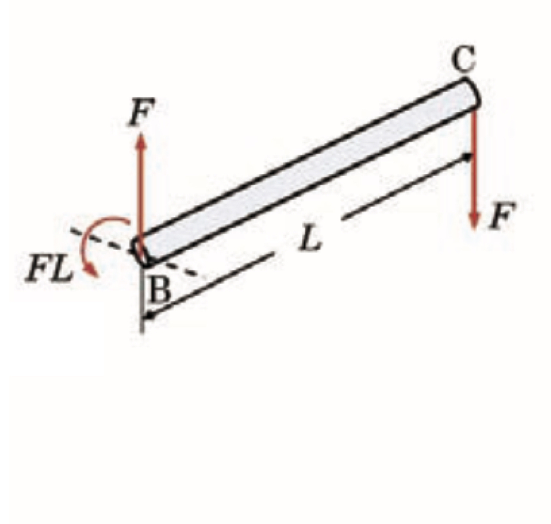
Fig. 10.16 Second (right) split off segment from the entire L shaped cantilever.#
We split the L-shaped cantilerver into a left ({see Fig. 10.15}) and a right (see Fig. 10.16) part. Regarding the left part we can assess that….
From the right part (see Fig. 10.16) we get
Now for \(\upsilon_v\)….
Where now these relations may be filled into \(\upsilon_c\) to find that
10.5. Additional Video#
This video by The Efficient Engineer provides a comprehensive visual breakdown of torsion in shafts. It begins with the fundamental definition of torque and demonstrates how it causes torsional deformation (angle of twist) and shear strain. A key focus is the derivation of the torsion formula (\(\tau = T\rho / J\)), which relates shear stress to the applied torque and the polar moment of inertia. The video also explores how to analyze shafts with multiple applied torques and explains the distinct failure modes for ductile and brittle materials under torsion. This video is non mandatory and is purely to give a different perspective on the topic.