2. Mechanics

2.1. Introduction

All man-made constructions (but also all natural structures) are under the influence of forces, temperature changes and vibrations. Sometimes such loads are constantly present and predictable, sometimes they occur sporadically and have a casual character.

A structure will deform as a result of loads. Excessive deformations can hamper functioning and lead to damage in the form of excessive wear and even breakage. When designing a structure, care must be taken that occurring deformations are small enough to ensure reliable operation and a sufficiently long service life. Predicting deformation caused by stress occurs with the help of theories and techniques from mechanics. It is essential here that people know how the material of which the construction is made behaves. This material behavior can be measured in a laboratory and then described with a material model.

A few concepts from mechanics will be introduced in this chapter. Furthermore, we will describe the material behavior of a typical steel type. Finally, we will see that for practical problems the use of computers and software is essential for predicting the mechanical behavior of a structure.

2.2. The rod: a one-dimensional construction element

In many constructions, machines and structures we can recognize parts that we can regard as a rod: a slender (long in one direction and short in the other directions) part that transmits a force in its longitudinal direction (= axial).

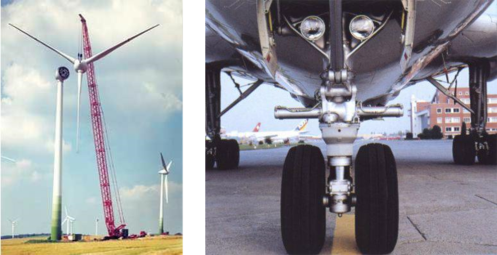
Fig. 2.1 Constructions with axially loaded parts.

The mechanical behavior of such a rod can be studied in the laboratory. A test is carried out with the aid of a tensile tester in which the rod is loaded in its longitudinal direction. The change in length due to the axial load is measured. We assume that the tensile bar in its initial condition has a length \(L_0\) and a cylindrical cross-section with surface \(A_0\). When the tensile bar is subjected to tensile load by an axial force F, the length will increase by \(L\) as outlined in Fig. 2.2 below.

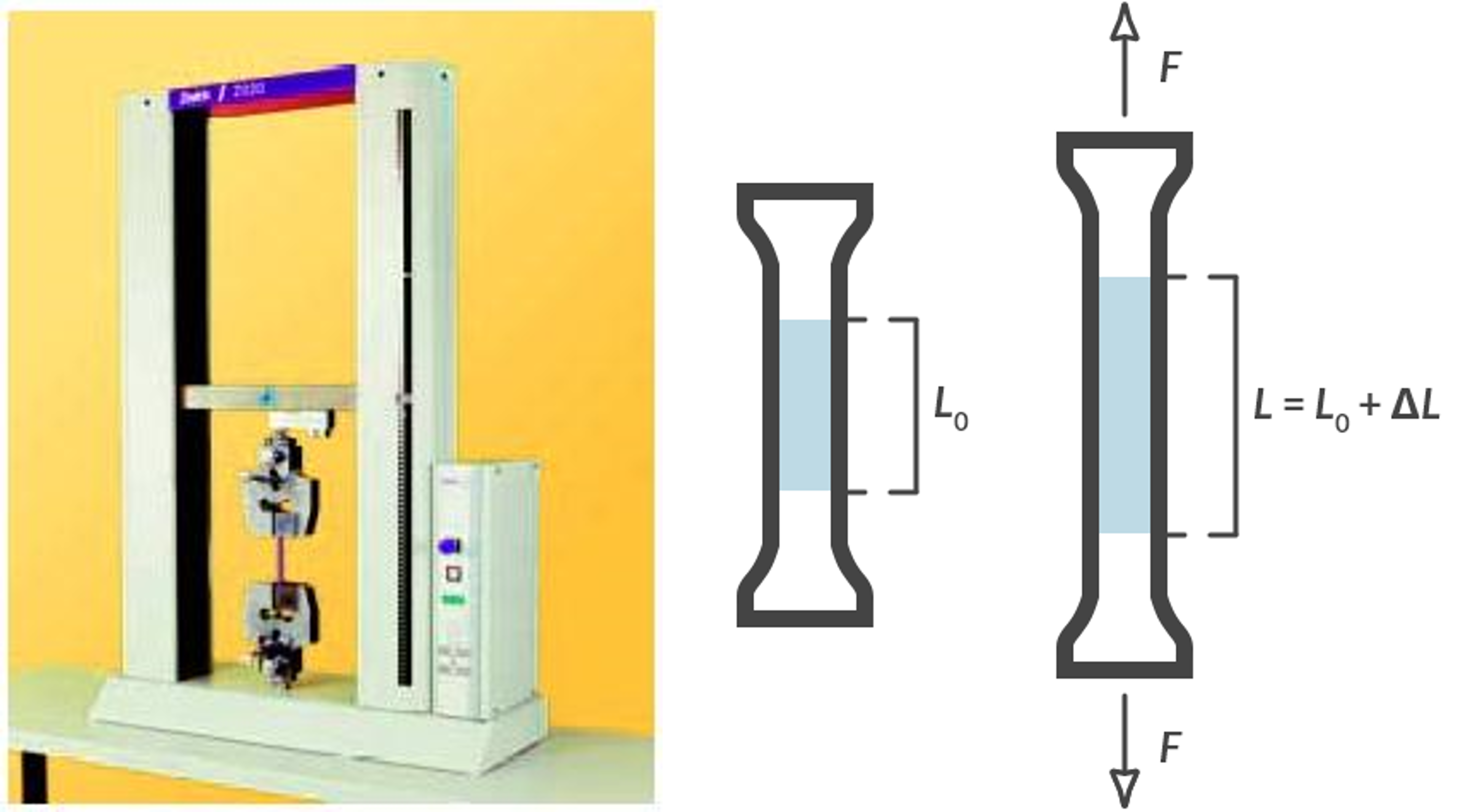
Fig. 2.2 (a) Tensile tester (source: Zwick), (b) tensile bar under load of a force \(F\).

If the extension is small, the relationship between \(F\) and \(\Delta L\) will be linear, therefore we can state:

(2.1)\[ F = k \cdot \Delta L \]

The proportionality factor \(k\) is called the stiffness of the bar. Experimentally it appears that the stiffness is proportional to the area of the cross-section \(A_0\) and inversely proportional to the length \(L_0\):

(2.2)\[ F = k(A_0, L_0) \cdot \Delta L \text{ with } k \propto A_0 \text{ and } k \propto \frac{1}{L_0} \to F = \frac{E \cdot A_0}{L_0} \cdot \Delta L\]

The parameter \(E\) appears to depend only on the material from which the bar is made and not on its dimensions. This material parameter is the elastic modulus.

By rewriting the above relationship, we see that the modulus of elasticity describes the linear relationship between and . These quantities play an important role. It is the nominal stress \(\sigma_n\) and the linear strain \(e\).

(2.3)\[ \frac{F}{A_0} = E \cdot \frac{\Delta L}{L_0} \to \sigma_n = E \cdot e\]

The linear relationship between \(\sigma_n\) and \(e\) indicates linear elastic material behavior and is known as Hooke’s Law. The word elastic indicates that, after the axial force has been removed, no permanent deformation of the rod can be measured: its length is again \(L_0\). Check this yourself.

Do you know the answer to the following question?

Robert Hooke (1635-1703) [1]

Robert Hooke FRS (18 July 1635 – 3 March 1703) was an English physicist (“natural philosopher”), astronomer, geologist, meteorologist and architect. He is credited as one of the first scientists to investigate living things at microscopic scale in 1665, using a compound microscope that he designed. Hooke was an impoverished scientific inquirer in young adulthood who went on to became one of the most important scientists of his time.[8] After the Great Fire of London in 1666, Hooke (as a surveyor and architect) attained wealth and esteem by performing more than half of the property line surveys and assisting with the city’s rapid reconstruction. Often vilified by writers in the centuries after his death, his reputation was restored at the end of the twentieth century and he has been called “England’s Leonardo [da Vinci]”.

Fig. 2.3 Portrait of Robert Hooke.

With a tensile tester we can also exert an axial pressure on the rod. According to agreement, the tension in the rod is then negative and that also applies to the strain that describes the shortening of the bar. For small negative strains, the relationship between n and \(e\) is described for almost all materials by the same elastic modulus \(E\) that we determined during the tensile test. We say that the linear elastic material behavior for tensile and pressure is identical.

If the length of the bar becomes longer or shorter during a tensile or compression test, the cross-sectional area will also change. It is clear that the bar becomes thinner with extension and thicker with shortening. For a rod with a circular cross section, we can indicate the thickness change with the diameter change \(\Delta D\). We can then introduce a new strain, the transverse strain ed,

(2.4)\[ e_d = \frac{\Delta D}{D_0}\]

With \(D_0\) the diameter of the undeformed rod. By accurately measuring the change in diameter, which is extremely small, during the tensile/pressure test, it appears that for linear elastic material behavior the following relationship exists between the transverse strain and the axial strain:

(2.5)\[ e_d = -v \cdot e\]

The material parameter \(v\) is called the Poisson ratio and is independent of the shape of the cross-section.

Elongation of a rod

A tensile force of 40000 N is applied to an aluminum rod with a diameter of 1.0 cm and a length of 2.0 meters. How far does the bar stretch? How much does the bar become thinner? See Table 2.1 for material data.

Solution

The following applies to the tension in the rod:

(2.6)\[ \sigma_n = \frac{F}{A_0} = \frac{F}{\frac{1}{4}\pi d_0^2} = \frac{40000}{\frac{1}{4}\pi (0.01)^2} = 5.09 \cdot 10^8 \textrm{ Pa} \]

With the modulus of elasticity of aluminum of 70 GPa the elongation becomes:

(2.7)\[ e = \frac{\sigma_n}{E} = \frac{5.09 \cdot 10^8}{70 \cdot 10^9} = 7.28 \cdot 10^{-3} \textrm{ [-]}\]

For a rod of \(2.0 \textrm{ m}\) this gives an extension of: \(\Delta L = L_0 \cdot e = 2.0 \cdot 7.28 \cdot 10^{-3} = 1.46 \cdot 10^{-2} \textrm{ m} = 1.46 \textrm{ cm}\).

The transverse strain is equal to: \(e_d = -v e = 0.21 \times 7.28 \cdot 10^{-3} = -1.53 \cdot 10^{-3}\).

After elongation the rod is \(\Delta D = e_d \cdot D_0 = -1.53 \cdot 10^{-3} \times 1 \textrm{ cm} = 1.53 \cdot 10^{-3} \textrm{ cm}\) thinner.

2.3. The stress-strain curve

Instead of the force ( stress), we can also prescribe the length change ( strain) of the test bar with a tensile tester. If the bar is extended, we can then register the stress-strain curve below.

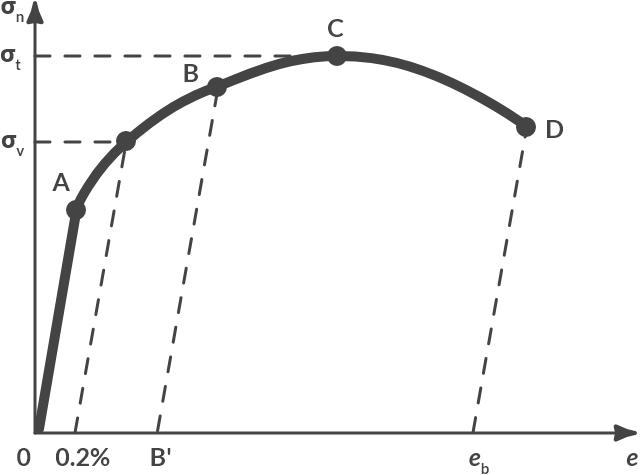
Fig. 2.4 Stress-strain curve for a typical steel alloy.

Up to point \(A\) there is linear elastic material behavior (\(\sigma_n = E \cdot e\)). From point \(A\), the relationship between \(\sigma_n\) and \(e\) is no longer linear. When in point \(B\) we let the tension become zero (= relieve), we can conclude that the test bar has undergone permanent extension: the material is plastically deformed.

When relieving pressure, the line \(BB\) ’is followed in the stress-strain curve, which turns out to be parallel to \(OA\). When loading again from point \(B\), we go up again past \(B’B\) until point \(B\) continues the initial stress-strain curve.

The stress at which the permanent (= plastic) elongation is 0.2% is called the yield stress of the material. Up to point \(C\), the stress increases with increasing elongation, a phenomenon called reinforcement. The maximum value of the stress that is reached in point \(C\) is the tensile strength \(\sigma_t\).

Upon reaching point \(C\), strange things happen to our test bar. The rod no longer remains nicely cylindrical but will start necking at a certain place, as can be seen in Fig. 2.5

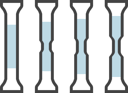
Fig. 2.5 Necking of a test bar.

In the neck, the cross-section will quickly become smaller with increasing elongation, while the other parts of the bar will hardly deform further. The tensile force \(F\) and the stress n will become smaller. In point \(D\), the rod is weakened by the increased neck so much that it breaks. The permanent plastic elongation after fracture is the fracture strain or elongation at break \(e_b\) .

The properties of materials can vary greatly. Table 2.1 shows the values of characteristic parameters for a few materials, which were determined by means of a tensile test and which were discussed above.

    

Britte (left) versus ductile and tough (right) behaviour of two polymers PS and PC, respectively.

Table 2.1 Characteristic parameters for some materials.

Material	\(E\) [GPa]	\(v\) [-]	\(\sigma_v\) [MPa]	\(\sigma_t\) [MPa]	\(e_b\) [-]
Steel	210	0.3	200	650	0.1
Stainless steel (type 304)	193		205	515
Cast iron	110			310
Copper	105			455
Aluminium (99.9%)	70	0.21		125	0.4
Titanium	110
Carbon fiber	230			3,800 - 4,200
Optical fiber	72.5	0.22		1,020
Polypropylene (PP)	1.14 - 1.55
Polyethylene (PET)	2.76 - 4.14		59	48.3 - 72.4
Polyvinylchloride (PVC)	2.14 - 4.14	0.38	40.7 - 44.8	40.7 - 51.7
Nylon 6.6	1.59 - 3.79	0.39
Rubber		0.5
Wood	12		108

The major differences in properties can be explained by considering the atoms and molecules that make up the materials and the way in which these building blocks are arranged.

2.4. Ashby Plots

An Ashby plot is a graphical tool used in materials science and engineering to compare and select materials based on their properties. It was developed by Michael F. Ashby to give engineers a systematic way to visualize large amounts of materials data. Instead of working through long tables of values, the data are represented on a chart where one material property is plotted against another, usually on double-logarithmic scales. Each family of materials, e.g., metals, polymers, ceramics, or composites, occupies a characteristic region or “blob” on the plot, reflecting the range of property values that are typically found in that group. An example of an Ashby diagram is presented in Fig. 2.6.

The purpose of an Ashby plot is to make material selection in design more intuitive and rigorous. Engineers often face conflicting requirements: a component may need to be strong but also lightweight, stiff but inexpensive, or heat-resistant but easy to process. By displaying the relevant properties together, the Ashby plot makes trade-offs visible and allows designers to identify which materials are promising candidates. For example, plotting strength against density can quickly highlight which materials offer high specific strength, a critical factor in aerospace and automotive design.

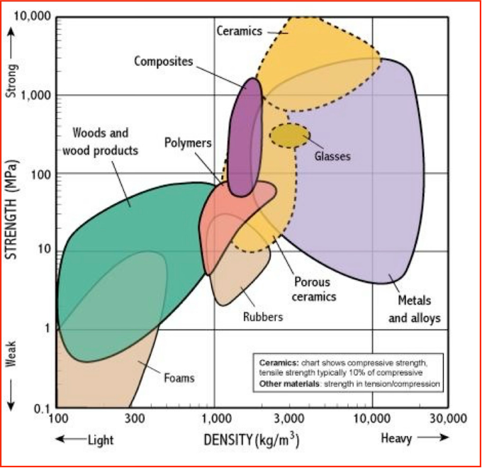
Fig. 2.6 Ashby diagram comparing different material classes on a strenght vs. density basis. Note that classes enclosed by drawn lines can be used both in tension and compression loading, while dashed-lines indicate suitability for compressive loads only.

Reading an Ashby plot involves a few steps. First, the engineer must identify the key design requirements of the component and express them as performance indices, i.e., combinations of material properties that measure how well a material meets a functional objective. The next step is to choose the appropriate property pair to plot, such as Young’s modulus versus density for stiffness-to-weight performance, or strength versus density for strength-to-weight performance as in the example of Fig. 2.6. On the chart, constraints can be drawn as boundary lines that separate feasible from non-feasible materials. These lines often represent constant values of a performance index. The materials whose regions lie within or near the feasible area become the shortlist of candidates. From there, more detailed considerations such as cost, processing methods, and availability can be used to refine the final choice. When a direct relation between the two material parameters can be established, this relation can be drawn on the log-log plot to determine the most suitable material class within the boundary conditions provided.

Ashby plots are most powerful in the early stages of design, when the range of possible materials is broad and the main goal is to narrow down the options efficiently. They allow quick elimination of unsuitable materials and highlight the few classes worth exploring in more depth. In this way, they provide both a visual overview of the material landscape and a structured pathway for decision-making in engineering design.

Michael F. Ashby (1935, age 89)

Michael Farries Ashby (see Fig. 2.7) is the British metallurgical engineer after whom Ashby plots are named. A former Royal Society Research Professor at the University of Cambridge’s Engineering Design Centre, he is renowned for his contributions to material selection through developing performance indices and graphical methods that aid rational design.

Ashby’s method reshaped the material selection process by combining material, feature, geometry, and processing considerations—using performance indices to narrow down candidates from databases of thousands of materials and visualizing them in Ashby charts. One of these charts can be seen in Fig. 2.6.

Fig. 2.7 Portrait of Michael F. Ashby in 2017.

2.5. Maximum allowable stress

In practice, it will usually not be permissible for a rod to deform plastically. The tensile/compressive stress occurring in the rod must therefore remain lower than the yield stress \(\sigma_v\).

2.5.1. Danger 1: Buckling

When a thin rod is loaded with a compressive force, the yield stress \(\sigma_v\) may not be reached. As everyone knows from experience, a thin bar will buckle under pressure loading, which is accompanied by large lateral displacement of points of the bar, as shown in the figure below. The force at which buckling occurs is the buckling load \(F_{\textrm{c}} \). The value of \(F_{\textrm{c}} \) depends on the way the bar is supported, but also on the shape of the cross-section, characterized by the second moment of area \(I\). For a circular cross-section, the following applies: \(I = \pi \cdot D^4/64\) and for a square \( (h \times h): I = h^4/12\). Fig. 2.8 shows how a bar bends for different supports. Table 2.2 shows the corresponding values of the buckling force \(F_{\textrm{c}} \).

Fig. 2.8 Buckling with various supports of a rod.

Table 2.2 Buckling load for various supports.

	1	2	3	4
\(F_{\textrm{c}} \)	\(\dfrac{\pi^2 E I}{L_0^2}\)	\(\dfrac{\pi^2 E I}{(0.7L_0)^2}\)	\(\dfrac{\pi^2 E I}{(0.5L_0)^2}\)	\(\dfrac{\pi^2 E I}{(2L_0)^2}\)

In Table 2.2, \(L_0\) is the starting length of the rod. After the rod has buckled, the stiffness will be greatly reduced, as shown in the figure. If the displacement \(u\) is not too large, the material behavior remains elastic and the rod will regain its original length when the compressive force is removed. In practice however, it will often happen that the displacement becomes too large and the rod breaks. Because of this and due to the fact that \(F_{\textrm{c}} \) often has a low value, buckling is a dangerous phenomenon that must be taken into account during the design of rod structures.

2.5.2. Danger 2: Fatigue

When the bar is subject to a load whose magnitude varies with time, the bar breaks over time, although the maximum stress is lower than the yield or buckling stress. This phenomenon is called fatigue. Experimentally it can be determined for a certain material how large the number of load changes to fracture, \(N_f\), is at a certain stress amplitude \(\Delta \sigma\) By carrying out the experiment for different values of \(\Delta \sigma\) a so-called (S-N)-curve can be determined, where \(S\) stands for \(\Delta \sigma\). A typical (S-N) curve is shown in Fig. 2.9.

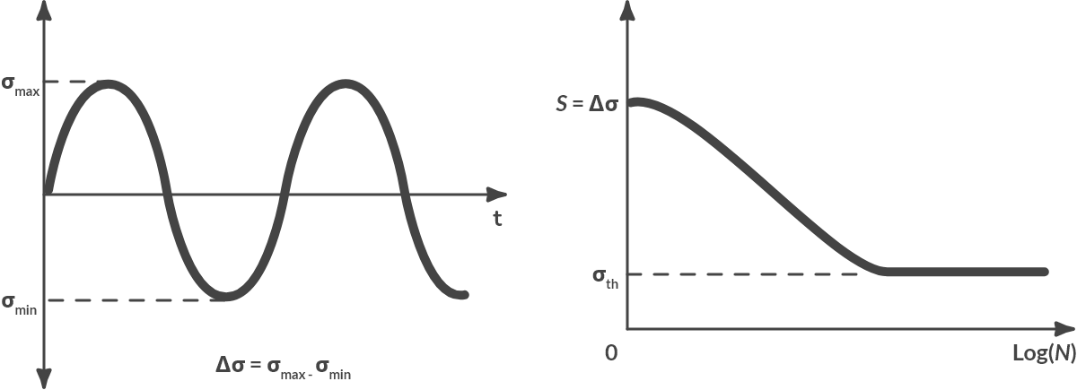
Fig. 2.9 Fluctuating stresses and (S-N)-curve (typical).

The number of load changes to breakage can be very large. For the drawn curve it is even the case that the lifetime becomes infinite when the stress amplitude remains below a limit value \(\sigma\)th. Fig. 2.10 shows the measured (S-N)-curves for several materials.

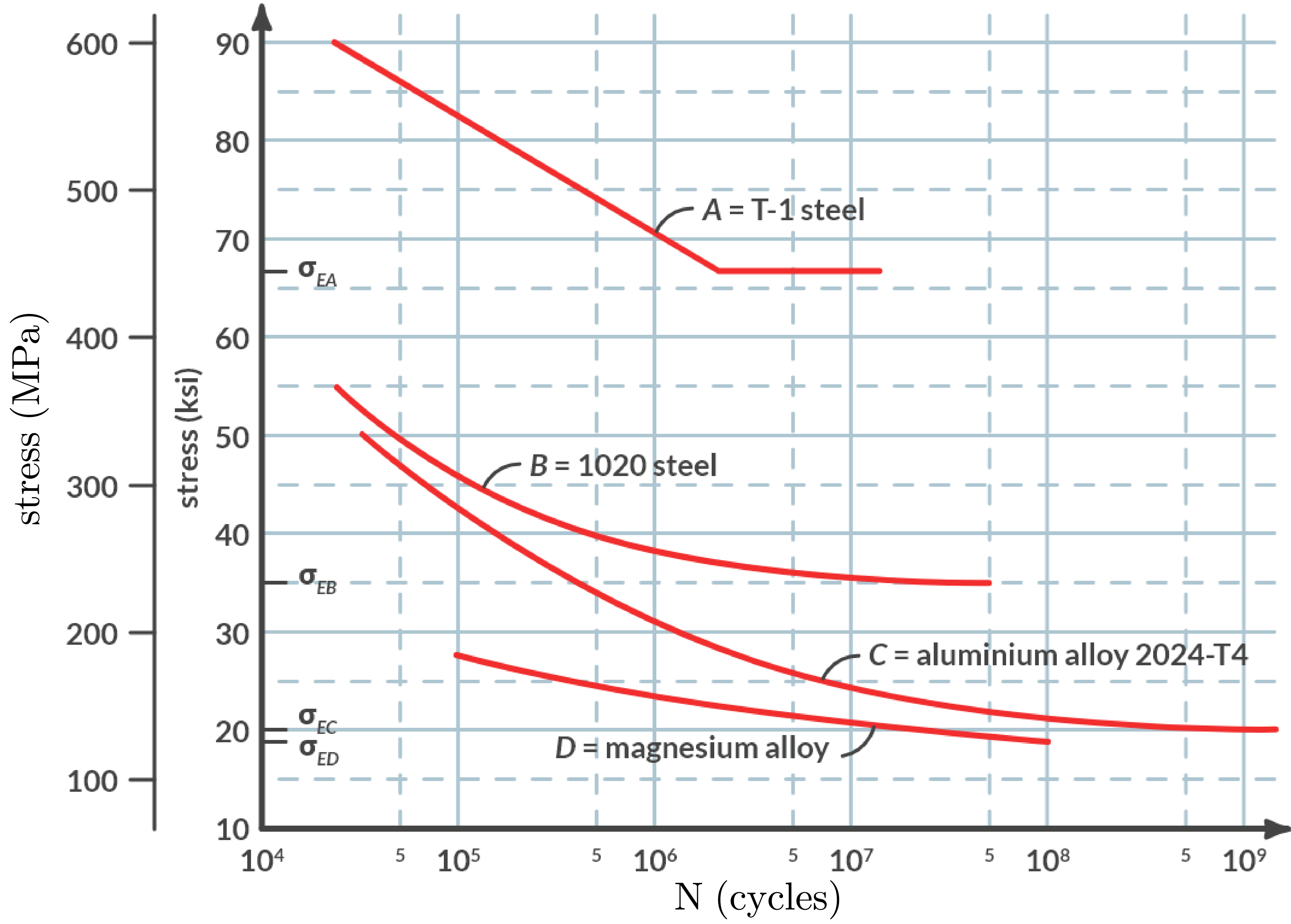
Fig. 2.10 (S-N)-curve for several materials.

Fortunately, such experimental data is readily available in the literature, so that we almost never have to perform such time-consuming experiments ourselves.

2.5.3. Safety factors

The calculation of deformations and stresses is based on mathematical models for equilibrium and material behavior. Model and material parameters must be determined through experiments. Results of model calculations and simulations cannot be fully trusted for the following reasons:

1. Simplifications in modeling. When formulating a model, reality is always simplified. As a result, no model will be able to describe reality with 100% accuracy.

2. Uncertainties in modeling. The properties of the materials from which a structure is constructed can differ from what is known or measured in a laboratory. Moreover, the measurement of material parameters is always done with finite accuracy.

3. Uncertainties in operating conditions. The (nature of) the actual load may be different from the load used for the calculations in the model. The conditions under which the structure must function can change the material properties.

Because of the uncertainties mentioned, safety margins are built in when designing structures. Calculation results are applied with a certain safety factor. Calculated limit values are adjusted downwards. The calculation models have improved considerably in recent years. More and more aspects of reality can be included in the modeling. This is mainly due to the considerably increased computing power of computers. The consequence of this is that the accuracy of the calculation results increases, and safety factors can decrease.

Bridge structure

Fig. 2.11 (a) shows a bridge truss structure that a small train (m = 2040 kg) must ride over. Fig. 2.11 (b) shows a schematic representation of this structure, for the situation where the train is in the middle of the bridge. The beams AB, BC, etc are all of the same length.

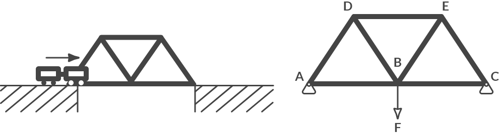
Fig. 2.11 (a) Construction of bridge with train (b) Schematic when train is in the middle.

For the situation where the train is in the middle of the bridge, the beam forces in the bridge have been calculated. These are given in the table below.

Table 2.3 Member forces in the truss structure of the bridge.

Member	\(F\) [kN]
AB	5.77
BC	5.77
CE	-11.55
DE	-20
AD	-11.55
BD	11.55
BE	11.55

The beams are connected to each other via pivot points. All beams are 6 meters long, have a round cross-section with a diameter of 0.05 meters and are made of steel.

1. Calculate the stress in each beam.

Solution

1. The stress in the beam can be calculated by \(\sigma = F/A\). All bars have the same cross-sectional area \(A = \pi D^2 /4 = 1.96 \cdot 10^{-3} \textrm{ m}^2\). The stresses thus become:

Table 2.4 Stresses in the beams.

Member	\(F\) [kN]	\(A\) [m\(^2\)]	\(\sigma\) [MPa]
AB	5.77	1.96 \(\cdot\) 10\(^{-3}\)	2.94
BC	5.77	1.96 \(\cdot\) 10\(^{-3}\)	2.94
CE	-11.55	1.96 \(\cdot\) 10\(^{-3}\)	-5.88
DE	-20	1.96 \(\cdot\) 10\(^{-3}\)	-10.19
AD	-11.55	1.96 \(\cdot\) 10\(^{-3}\)	-5.88
BD	11.55	1.96 \(\cdot\) 10\(^{-3}\)	5.88
BE	11.55	1.96 \(\cdot\) 10\(^{-3}\)	5.88

2. Is the maximum allowable tensile stress achieved in one of the beams?

Solution

2. The maximum tensile stress of steel is 650 MPa (see Table 2.1). This stress is not achieved in any of the elements.

3. Can this bridge bear the load? Explain!

Solution

3. Although the maximum tensile stress is not exceeded, there is a risk of buckling. As all bars are connected to each other via hinges, buckling variant 1 (see Fig. 2.8) can occur. The following applies to the buckling force of buckling variant 1:

(2.8)\[ F_{\textrm{c}} = \frac{\pi^2 E I}{L^2} = \frac{\pi^2 \times 207 \cdot 10^9 \times 3.07 \cdot 10^{-7}}{6^2} = 17.5 \textrm{ kN}\]

The second moment of inertia I for a circular rod is equal to: \(\pi \cdot D^4/64 = 3.07 \cdot 10^{-7} \textrm{ m}^4\).

The modulus of elasticity \(E\) for steel is equal to 210 GPa (see Table 2.1).

Buckling only occurs in bars with compressive stress. If we look at the negative beam forces (compressive forces) in Table 2.3, it is striking that that buckling force is achieved in bar DE. That is why the bridge probably cannot bear the load on the train!

2.6. What lies ahead

In this chapter a number of concepts are described, which play an important role in mechanics. Attention is initially focused on an axially loaded structural element, the rod, which can only transmit a force along the rod axis, which only results in an axial tension. There are also one and two-dimensional parts that can guide bending moments and torques: beams and shells. Finally, there are three-dimensional elements that can transmit forces and torques in three directions.

External load leads to deformation, which is described (and also measured) as strain. For linear elastic material behavior, there are very simple relationships between occurring stresses and strains. For most constructions it is important that the stresses remain as low that the material behavior remains linearly elastic. Permanent deformation is unacceptable.

External circumstances can lead to the material behavior no longer being linearly elastic. At high loads, most materials will deform plastically (= permanently). Plastics will also exhibit viscoelastic behavior under low loads, where the loading speed plays an important role. With metals, a similar effect occurs when the temperature is high. Mathematical models have been formulated to describe all these forms of material behavior. Experimental techniques have been developed to determine the often many material parameters.

Mechanical calculations are frequently used to describe the large plastic deformations that occur with increased stresses. This is particularly the case when analyzing design processes such as rolling, forging, extruding, sheet processing and machining, whereby the aim is often to optimize process conditions. Finally, it is becoming increasingly important to be able to predict what will happen if there is damage (a crack) in the material. If a component fails, it is not desirable for the entire structure to collapse, with all its consequences.

It goes without saying that numerical calculations with the computer play an increasingly important role in predicting the mechanical behavior of structures and materials. Although much software is now commercially available, improved analysis methods and material models are constantly being translated into reliable and efficient software. Programming techniques and knowledge of numerical methods and information processing therefore play an important role in mechanics. Not only in solid mechanics, but also in fluid mechanics.

2.7. Problems

For the following exercises use symbols as long as possible and only in the end fill in the values given.

Exercise 2.1 (Space tower)

Inspired by a first-year Bachelor course a student got the idea to build a space tower. From the roof of this tower space ships could be launched. The student has the great idea to make the tower high enough such that space ships would need less fuel to be launched. The students ambition is illustrated in Fig. 2.12 below.

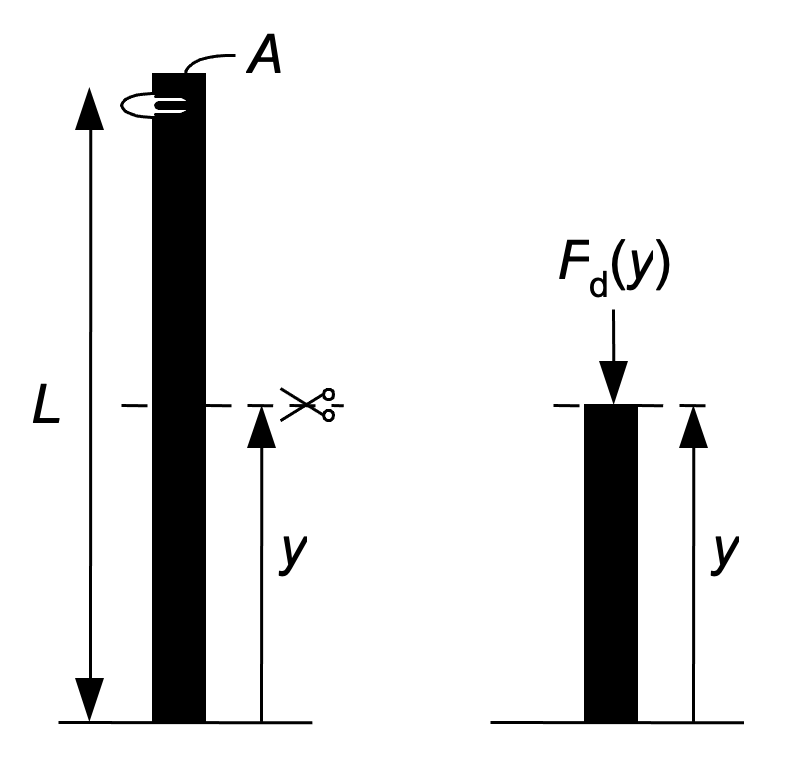
Fig. 2.12 Schematic drawing of the space tower (left), cross section at height \(y\) meter (right).

As a first estimate to determine how higher the tower should be the student starts with a simple design. Assumed is that the is massive, round and with a fixed diameter \(D\) and cross-sectional area \(A\) with length \(L\). For the material properties of the tower the student defines a density \(\rho = 7850\) kg\(/\textrm{m}^3\), elasticity modulus \(E = 207\) GPa and yield stress \(\sigma_{\text{v}}= 400 \) MPa. We consider the cross section at height y meter, as in Fig. 2.12. In addition, we assume that gravity is constant for any height \(y\)

1. Show with clear steps that for the compression force \(F_{\textrm{d}}(y)\) for the bottom part of the tower holds

\[ F_{\textrm{d}}(y) = \rho A g(L-y) \]

Table 2.5 Parameters space tower

	Parameters
\(F_{\textrm{d}}(y)\)	compression force for the bottom part of the tower [N]
\(\rho\)	density of the material [kg\(/\textrm{m}^3\)]
\(A\)	area of the cross section of the tower [\(\textrm{m}^2\)]
\(g\)	gravity [\(\textrm{m}/ \textrm{s}^2\)]
\(y\)	height of the bottom part of the tower [\(\textrm{m}\)]
L	the total length of the tower [\(\textrm{m}\)]

2. Determine at which position \(y\) the compression force in the tower is maximum.

Constructions that are loader under compression rarely collapse due to exceeding the yield stress. The chances are much larger that the construction will fail due to buckling. This configuration is shown in Fig. 2.13.

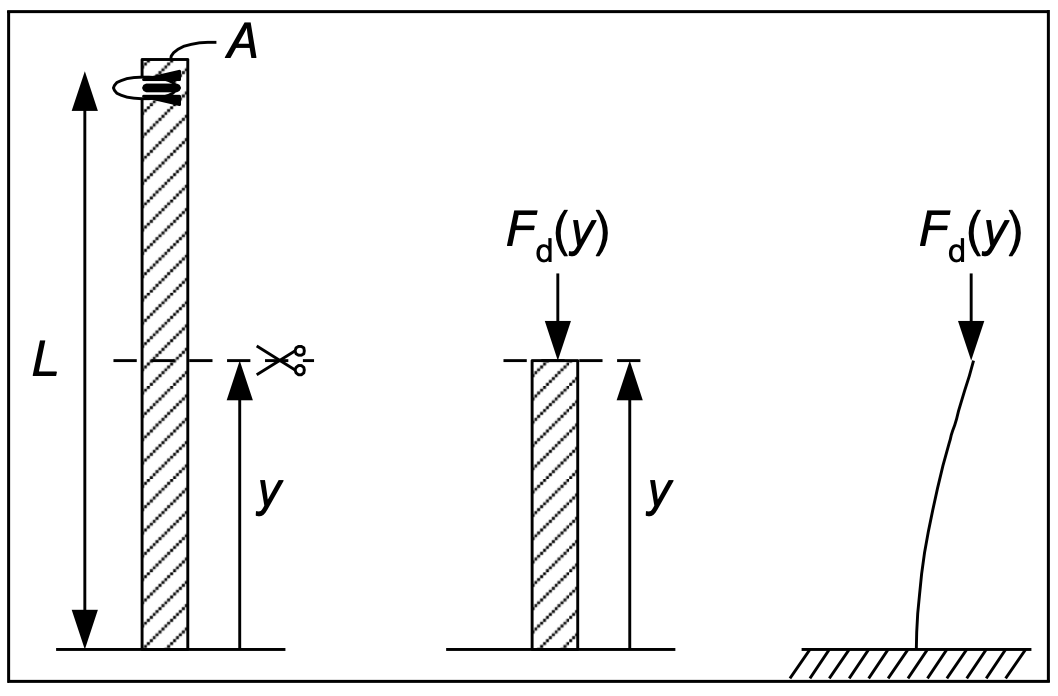
Fig. 2.13 Schematic representation of the space tower for buckling analysis.

As of this point we assume that the massive round tower a diameter of \(D = 4\) m with a length \(L = 1000\) m. The material properties are: \(E = 207\) GPa, \(\rho = 7850\) kg\(/\textrm{m}^3\) and \(\sigma_v = 400\) MPa. We again consider the cross section at height \(y\) meters and consider the tower as an element with a fixed support in the earth, see Fig. 2.12.

3. Where is the risk of buckling the largest? Around \(y \approx 0\) m, \(y \approx 1/2\)L m or \(y \approx\)L m? Explain your answers!

4. Find an expression for the maximum allowable buckling force \(F_{\text{kn}}(y)\) that can carry the load of the tower under a cross section at height \(y\).

5. Compute the maximum allowable buckling force \(F_{\text{kn}}\) and the compression force \(F_{\textrm{d}}\) for \(y = 50\) m.

With a graphical calculator we draw in an \(F-y\) diagram the maximum allowable buckling force \(F_{\text{kn}}\)(y) maximum allowable buckling force \(F_{\textrm{d}}(y)\) as a function of \(y\) for \(0 \leq y \leq 200\). The results of the graphing are shown in Fig. 2.14.

Fig. 2.14 Maximum allowable buckling force and compression force for a steal space tower of \(1000\) m.

6. Will the tower fail due to buckling? Explain!

Context

Space travel occurs nowadays most with rockets. In the past also space shuttles were used. Fuel consumption is a major expense and most of the fuel is needed during lift-off. A space elevator would make it possible to launch space ships from a large altitude such that gravity has much less influence.

The space elevator consists of a geostationary space station that at an altitude of \(36000\) km height orbits around the earth. With the use of a lift cabin one would be transported from earth to the space station. In Fig. 2.15 a (virtual) picture is shown of the space elevator from the space station.

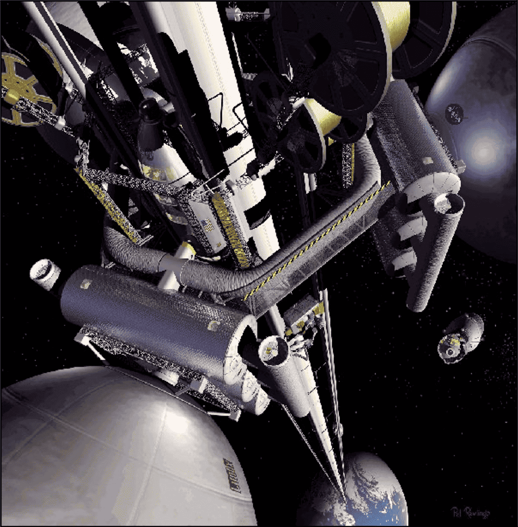
Fig. 2.15 Image of the space elevator from the space station.

Already in \(1966\) American scientists explored the idea of a space elevator and started with some first calculations. At this moment, NASA is still looking into options for such a space elevator. At this moment such a space elevator is not feasible, but they expect that with \(50\) years it will be technically possible.

Research and design questions

A number of different questions play a role when considering a space elevator as an replacement for rockets.

• What load should the cable bear?

• Which material properties play a role?

• Is there a material that is suitable for this?

• Are there ideas for reducing the load?

Exercise 2.2 (Space elevator I)

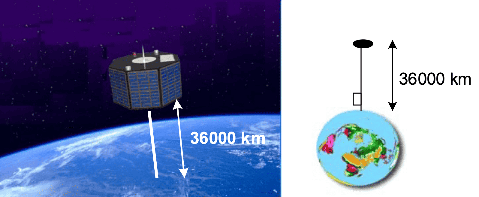
Fig. 2.16 Schematic view of a space elevator.

At the space station (at \(36000\) km above the Earth’s surface) the cable must carry the mass of the lift (plus content) and carry its own mass. Suppose that the force of attraction (gravity) is not a function from the distance to the earth, but that it is constant.

Make a drawing of the (cylindrically assumed) cable with the space elevator at the top end and add the following given parameters:

• height \(H\) of the entire cable

• cross-sectional area \(A\) of the cable

• height \(y\) at which we imaginary cut the cable

• mass \(m\) of the entire cable

• mass \(M\) of the space lift

• gravity constant \(g\)

• elastic modulus \(E\) of the cable material

• density \(\rho\) of the cable material

1. Calculate the mass \(m\) of the cable if we use a steel cable (\(\rho = 7858\) kg\(/\textrm{m}^3\)), with a cross-section \(A\) of \(1.00 \textrm{ cm}^2\). Assume that the lift plus content weighs \(10000\) kg.

2. Is this load negligible in relation to the own weight of that cable?

We neglect the weight of the lift plus content.

3. Calculate the gravity \(F_{\textrm{g}}\) of a cable of length \(y\) [m].

4. Derive an expression of the nominal stress \(\sigma_n\) in the cable as function of the height \(y\) With \(\sigma_n\) in [N\(/\textrm{m}^2\)] and y in [m]. What do you notice?

5. What is the maximum allowable stress in the cable if we were to make the cable from steel? At what height is that stress (already) achieved?

A better material to use would be a high molecular weight fiber polyethylene. The strongest fiber that is available has a tensile strength of \(9\) GPa and a density of \(1000\) kg\(/\textrm{m}^3\).

6. Compute the height that can be achieved with this material.

7. Which two material properties are finally determining the achievable height?

Exercise 2.3 (Space elevator II)

One of the solutions that NASA suggested at the time was a tapered cable. The diameter of the cable increased as you were further away from the earth.

1. Explain why that is quite a smart idea.

One of the solutions for the cross-section A as a function of the distance h to the earth’s surface is

\[ A(h) = A_{\text{max}}\cdot \frac{h}{36000\cdot 10^3} \, [\textrm{m}^2].\]

2. Draw the cross section \(A\) and the radius \(R\) (starting from a round cable) as a function of the height \(h\) [m].

3. Calculate the volume \(V\) (y) of a cable with length \(y\) that starts from the earth’s surface.

4. Determine an expression for the stress \(\sigma\) in the cable as a function of the height \(y\) [m].

5. Calculate what height we now reach with steel? And with the aforementioned polyethylene fiber?

Exercise 2.4 (Space elevator III)

We now abandon the assumption that gravity \(F_{\textrm{g}}\) is constant. In reality, gravity decreases as we move further away from the earth. For the gravity \(F_{\textrm{g}}\) (h) of the earth mass \(M\) on an object \(m\) that is at height \(h\) [m] of the earth’s surface,

\[ F_{\textrm{g}}(h) = G M \cdot \frac{m}{(h+r)^2} [N] \]

applies. Table 2.6 below gives the parameters for this exercise.

Table 2.6 Parameters space elevator III

	Parameters
\(F_{\textrm{g}}(y)\)	the gravity on an object at height y in [N]
m	the mass of the object in [kg]
\(G\)	the gravitational constant in [\(\textrm{m}^3/\textrm{s}^2\, \textrm{kg}\)] \((66,7\cdot 10^{-12} \,\textrm{m}^3/\textrm{s}^2\, \textrm{kg})\);
\(M\)	the mass of the earth in [kg] \((5,976\cdot 10^{24} \textrm{ kg})\)
\(r\)	the radius of the earth in [m] \((6,378\cdot 10^6 \textrm{ m})\)
\(h\)	the distance from the object to the surface of the earth in [m]

1. Determine a function for gravity \(F_{\textrm{g}}\)(y) on a cable, with a constant cross section \(A\) and length \(y\), it starts on the earth’s surface.

2. Determine an expression for the stress \(\sigma_n(y)\) in the cable at height \(y\).

3. Calculate how high we are now with steel? And with the polyethylene fiber?

You can see that the effect of decreasing gravity only becomes noticeable at large distances from the earth. With steel the effect is negligibly small, with polyethylene fiber it saves more than 10%! There are currently developments in the field of super strong and super light materials.

Exercise 2.5 (Buckling load of a plastic ruler)

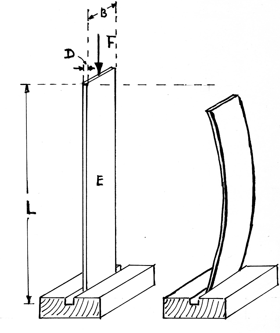
Fig. 2.17 Plastic ruler in gutter; loaded vertically.

A plastic ruler in a gutter is illustrated in Fig. 2.17. To demonstrate buckling, a standing plastic ruler is considered with modulus of elasticity \(E\), which is placed at the bottom in a narrow channel (to prevent slipping) and which is pressed down vertically from above. The rotation on the underside is free, so that the buckling situation on the left from Fig. 2.8 may be assumed. Assume a length \(L\), a thickness \(D\) and width \(B\) (all in m).

1. Calculate the buckling force \(F_{\text{c}}\) parametrically.

2. Make realistic assumptions for the values of the unknown (required) parameters.

3. Calculate the number value and therefore the order size of \(F_{\text{c}}\).

4. Calculate the nominal pressure in that ruler.

Exercise 2.6 (Material Properties)

In this assignment we will look at some practical aspects of the choice of materials. For this we consider the design of a simple beam (for example a beam of the frame of an aircraft) which is loaded longitudinally (uniaxially), see Fig. 2.18.

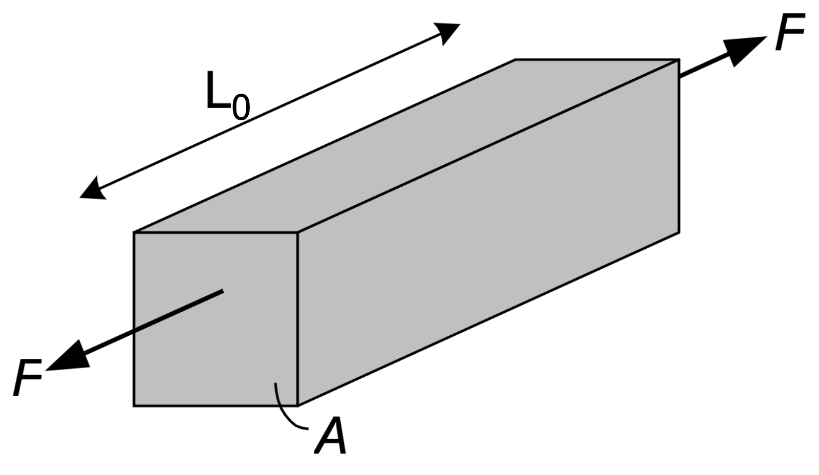
Fig. 2.18 Uni-axially loaded beam

The beam has a square cross section \(A\) and a length \(L_0\). The intention is to determine the required transverse area A for different materials, such that the beam acquires a stiffness k of \(10^8\) N/m. The materials that we are going to compare are steel, wood, polyvinyl chloride (PVC) and silicon carbide (SiC).

The required data for these materials is shown in the table in Table 2.7.

Table 2.7 Mechanical material propertiies.

Material	Modulus E [GPa]	Allowable tensile stress \(\sigma_t\) [Mpa]	Allowable pressure \(\sigma_p\) [MPa]	Density \(\rho\) [\(10^3 \textrm{ kg}/\textrm{m}^3\)]	Material cost \(C_r\) [\(\$/\textrm{kg}\)]
Steel	\(210\)	\(200\)	\(200\)	\(7.8\)	\(2.7\)
Wood	\(10\)	\(100\)	\(75\)	\(0.48\)	\(1.7\)
PVC	\(3\)	\(50\)	\(52\)	\(1.2\)	\(1.25\)
SiC	\(400\)	\(1\)	\(8000\)	\(3\)	\(66.7\)

Recall:

• \(1\, \textrm{ Pa} = 1\, \textrm{ N}/\textrm{m}^2\)

• \(1\, \textrm{ MPa} = 1\cdot 10^6\, \textrm{ N}/\textrm{m}^2 = 1\, \textrm{ N}/\textrm{mm}^2\)

• \(1\, \textrm{ MPa} = 1\cdot 10^6\, \textrm{ N}/\textrm{m}^2 = 1\cdot 10^3\, \textrm{ N}/\textrm{mm}^2\)

• \(1\cdot 10^3 \textrm{kg} = 1\) ton mass

1. Show with a clear step-by-step calculation that the required cross-section \(A_0\) is given by

\[A_0 = \frac{k L_0}{E}.\]

Table 2.8 Parameters

	Parameters
\(A_0\)	The cross section in [\(\textrm{m}^2\)]
\(k\)	The stiffness in [N\(/\textrm{m}\)]
\(L_0\)	Entrance lenght of the beam in [\(\textrm{m}\)]
\(E\)	Elastic modulus in [Pa]

2. Show that the required cross-section for a wooden beam would be \(10 000 \textrm{mm}^2\) per unit lenght. Then calculate the required cross sections if the beam is made of steel, PVC or SiC.

3. Now calculate the total mass of the beam for the four mentioned materials. Which beam is the lightest?

4. With the data from Table 2.7 you can also estimate the material costs for each beam. Which beam is the cheapest?

5. Calculate the force in kN if the beams are loaded under tension.

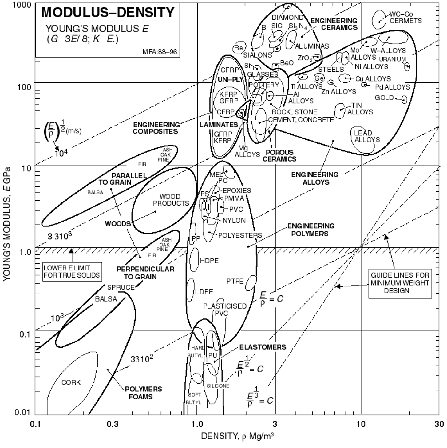
Fig. 2.19 Ashby-plot: Elastic modulus \(E\) versus density \(\rho\).

If one desires to design a beam with a certain stiffness and not exceed a certain mass, one can use the so-called Ashby plots. In Fig. 2.19 the Ashby plot is given for Elastic modulus \(E\) versus density \(\rho\) . The graph also contains “guidelines for minimum weight design”. One of the lines is : \(E/\rho = \textrm{Constant}\).

6. Check if the density and elastic modulus of the materials from Fig. 2.18 match with the Ashby-plot from Fig. 2.19. Indicate in the Ashby-plot where these materials can be found.

7. Show that with designing for stiffness the mass of the beam will always be the same for all materials where \(E/\rho\) has the same value.

8. In the graph of Fig. 2.19 several lines for a constant \(E/\rho\) are given. Does a higher value of \(E/\rho\) lead to a lighter or heavier beam? Check with the aid of these lines if the order of the beam masses from exercise \(3\) matches.

Exercise 2.7 (Beams that can carry the same buckling load)

As an example, we are going to spend some more time on a compression loaded beam, see Fig. 2.20. We again assume that the beam has a given constant length \(L_0\) and a square cross section \(A_0\).

Fig. 2.20 Compression loaded beam.

1. Show that if the beam is dimensioned on an equal buckling load, the cross section \(A_0\) is given by the formula below.

Use the buckling formula (variant 1) from Table 2.2:

\[ A_0 = \sqrt{\frac{12 F_{\textrm{c}} L_0^2}{\pi^2 E}}. \]

Table 2.9 Parameters

	Parameters
\(A_0\)	The cross section in [\(\textrm{m}^2\)]
\(F_{\textrm{c}} \)	The buckling load in [N]
\(L_0\)	The initial length of the beam in [\(\textrm{m}\)]
\(E\)	Elastic modulus in [Pa]

2. Show that when designing on articulated load the mass of the beam will be the same for all materials for which \(\sqrt{E}/\rho\) has the same value.

3. Use an Ashby plot again, now in Fig. 2.21, and determine which of the four materials (steel, wood, PVC and SiC) would provide the lightest beam for a given maximum buckling load.

Fig. 2.21 Ashby-plot: Elastic modulus \(E\) versus density \(\rho\).

Exercise 2.8 (Bridge construction)

We consider a simple bridge construction intended for road traffic. The bridge construction is (schematically) shown in Fig. 2.22.

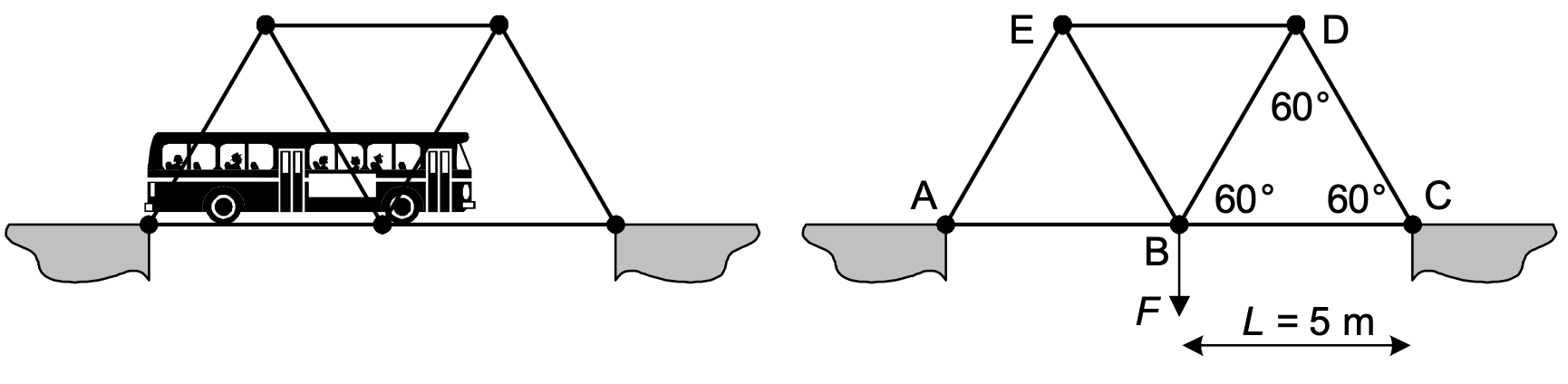
Fig. 2.22 (left) Bridge construction, (right) schematic representation.

A bridge element that is subjected to tensile stress and concentrate on the choice of material for the bar is concidered. In the first instance, two options are assumed: structural steel and lightweight wood. The following data in Table 2.10 is known for both materials.

Table 2.10 Bridge construction

Material	Modulus E [GPa]	Allowable tensile stress \(\sigma_t\) [Mpa]	Density \(\rho\) [\(10^3 \textrm{ kg}/\textrm{m}^3\)]	Material cost \(C_r\) [\(\$/\textrm{kg}\)]
Construction steel	\(210\)	\(200\)	\(7800\)	\(2.7\)
lightweight wood	\(10\)	\(100\)	\(480\)	\(1.7\)

The bridge element that is subjected to tensile stress has a length \(L = 5\) m, a round section A and must be able to withstand a tensile force \(F_t\) of \(50\) kN (see Fig. 2.22). The load due to own weight does not have to be taken into account.

1. For both materials, calculate the cost of a rod that can withstand the said tensile force. Which yields the cheapest bridge element?

2. Show that the material cost \(K_{\textrm{m}}\) is given by

\[ K_{\textrm{m}} = \rho\, C_m \frac{F}{\sigma_t}\, L.\]

Table 2.11 Parameters

	Parameters
\(\rho\)	The density of the materialin [kg\(\textrm{m}^3\)]
\(C_r\)	The cost of the material in [\(\$/\textrm{kg}\)]
\(F\)	The tensile load in [N]
\(\sigma_t\)	The length of the beam in [m]

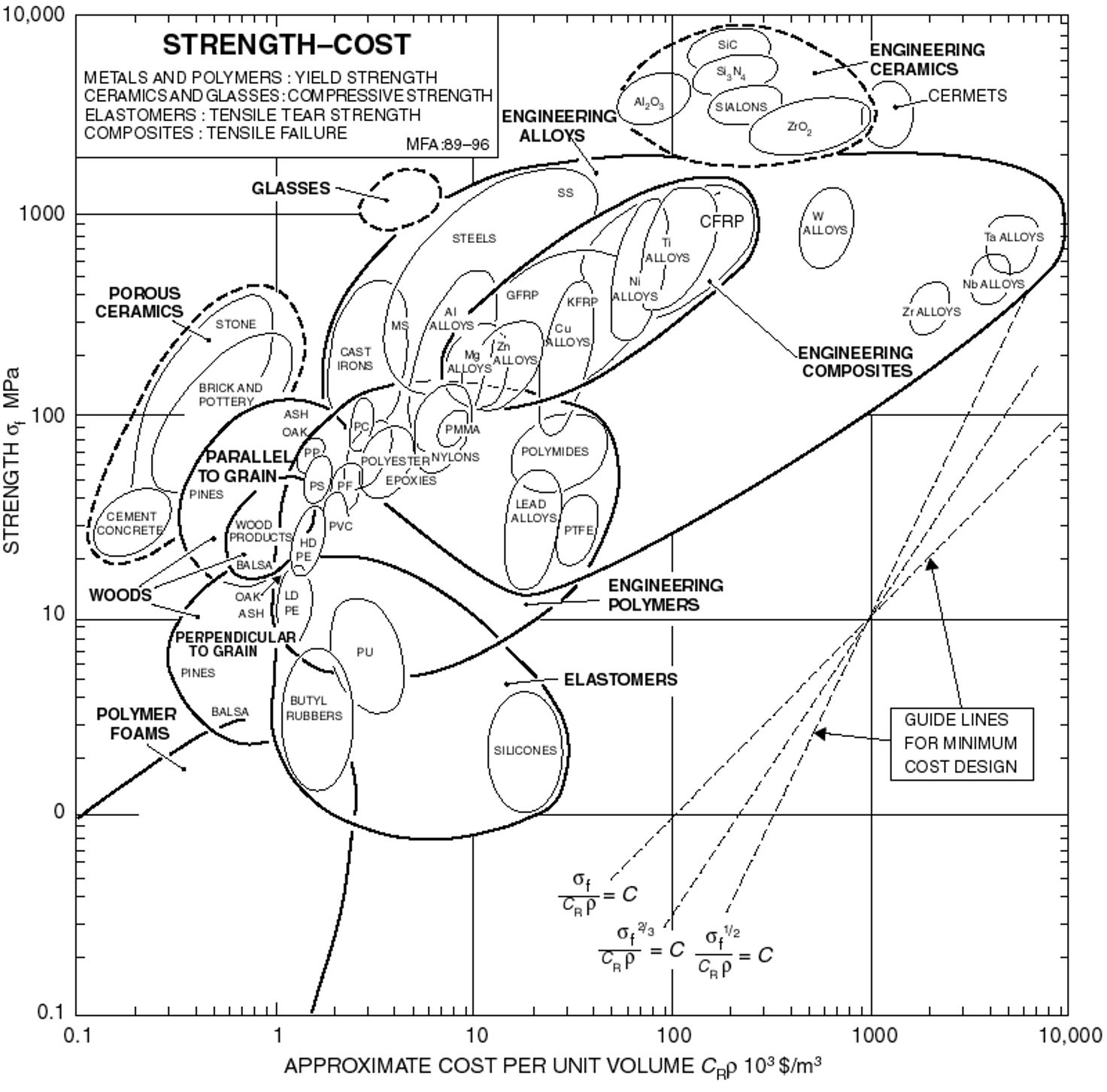
Fig. 2.23 Ashby-diagram, strength versus material cost.

3. In Fig. 2.23 you see an Ashby-plot of \(\sigma_f\) (\(\sigma_t\) in our case) against \(C_r\rho\). one of the lines is the line given by

\[ \frac{\sigma_t}{C_r\rho} = C.\]

Explain that for each material in such a line the costs for the bridge elements are the same.

4. Determine the material that yields the cheapest beam from the Ashby plot in Fig. 2.23. Explain clearly how you work. Support your explanation graphically in the Ashby plot.

Exercise 2.9 (Waferstepper stage)

Modern chip manufacturing relies on EUV lithography for the most accurate parts of the chip. One of these machines may be seen in Fig. 2.24. Unfortunately, almost all substances (including air) significantly absorb EUV photons which requires all sorts of systems to be placed in vacuum. In general, realizing mechatronics systems in vacuum is significantly more expensive than ambient conditions: it requires expensive pumps, polymeric materials are typically not compatible, and the heat generated in the actuators is not cooled down because there is no air convection (see Section 4).

Fig. 2.24 A view of a wafer stepper system used in EUV lithography. The animation highlights the complex vacuum chamber and surrounding mechatronic components required for high-precision chip manufacturing.

To simplify the mechatronics system, we investigate a concept where the positioning stage is driven from outside the vacuum vessel. The stage as may be seen in Fig. 2.25 with mass \( m= 100\,\)kg is driven from the outside using a steel rod with radius \(r\), length \(l=500\,\)mm, Young’s modulus \(E=210\,\)GPa and yield strength \(\sigma_y=200\,\)MPa. At the base of the rod a force \(F\) is exerted and the position \(\varphi\) is measured.

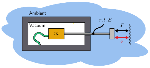
Fig. 2.25 Conceptual diagram of the proposed external actuation setup. A steel rod with radius \(r\), length \(l\), and material properties \(E\) and \(\sigma_y\) transmits a force \(F\) from outside the vacuum vessel to drive the stage of mass \(m\), while the displacement \(\varphi\) is measured.

To meet the productivity requirements, we are required to drive the stage with a peak acceleration of \(100\,\textrm{m}/\textrm{s}^2\). Our mission is to choose an appropriate radius that meet this, and later other requirements.

1. When moving the stage to the right, the rod is loaded in tension. How large does the radius at least need to be for a stainless-steel rod? What about aluminum (find the representative values for aluminum yourself)? You can neglect the mass of the rod for load calculations.

2. Does the previous result still hold when we move the stage in the other direction? Justify and, if needed, provide the new minimum radius for both materials.

3. In reality, this movement is made many times per production step. How many cycles will the rod be able to withstand before it fails?

---

[1]

https://en.wikipedia.org/wiki/Robert_Hooke