6. Control

6.1. Introduction

Control is a common term, used in many biological, business, economic and technical systems. In this chapter we will discuss several basic concepts and choose applications from mechanical engineering practice. Some examples of such applications are:

• the central heating thermostat (temperature control),

• the cruise control of a car (velocity control)

• the float in a toilet (level control),

• the EUV positioning,

• an autonomous warehouse robot.

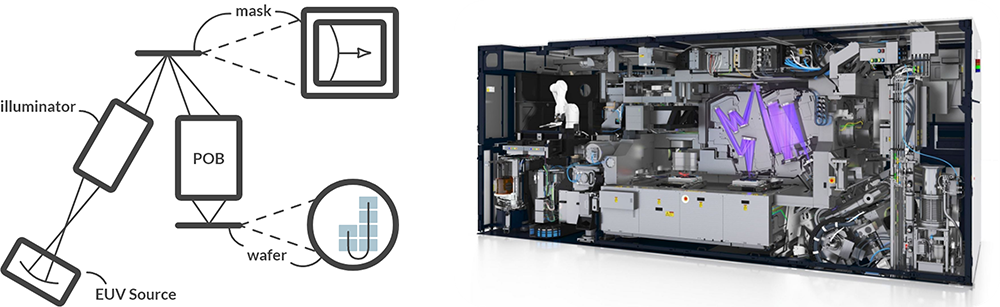
Fig. 6.1 (a) Schematic representation of an EUV, (b) EUV Positioning (source: ASML).

Control technology plays a role in all these examples. In short, you could say that control engineering is concerned with the design and implementation of “controllers” that ensure that certain variables of a device retain a desired value or follow a desired trajectory (as a function of time). In a somewhat broader sense, the discipline also pays attention to modeling the dynamic behavior of systems, for instance through experiments, the analysis of signals and disturbances, and the design of control signals or controls in the form of feedbacks. In this chapter we will briefly discuss the block diagram notation, the principle of the feedback control and an analysis of a simple regulated system.

6.2. Signals and systems

In control technology, systems are displayed with the so-called block diagram notation. In the block diagram notation, a system is seen as a set of block functions that are connected with arrows. Signals (variables) pass over the arrows. These are quantities that are a function of time. Each block function has an input and an output. The block function describes the relationship between that input and output. Fig. 6.2 shows two basic building blocks.

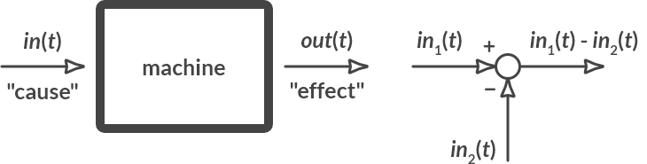
Fig. 6.2 Basic elements of a block diagram.

On the left you see a block function. This function usually contains a dynamic model, described with a differential equation. On the right you see a summation node. At the summation point, a minus sign indicates that the relevant signal must be subtracted. If there is a plus sign, or if there is nothing, the corresponding signal must be added. In Fig. 6.2 the output signal is therefore equal to \(\textrm{in}_1(t)-\textrm{in}_2(t)\).

The identification of which signal is to be regarded as the input of a system and which signal is to be regarded as the output is usually self-evident. In principle, a logical “cause \(\rightarrow\) effect” relationship must be maintained, which then corresponds to “input \(\rightarrow\) output”. There are circumstances where the cause-effect relationship is not entirely clear and where multiple choices can be made. In this first orientation in the field, cases will be considered that have a clear cause-effect relationship.

Fig. 6.3 shows several examples of a block diagram. You see that you can draw different block diagrams from the same system. For example, you can break down some complex block functions into two simpler block functions. This is done, for example, with the pulley in Fig. 6.3(b).

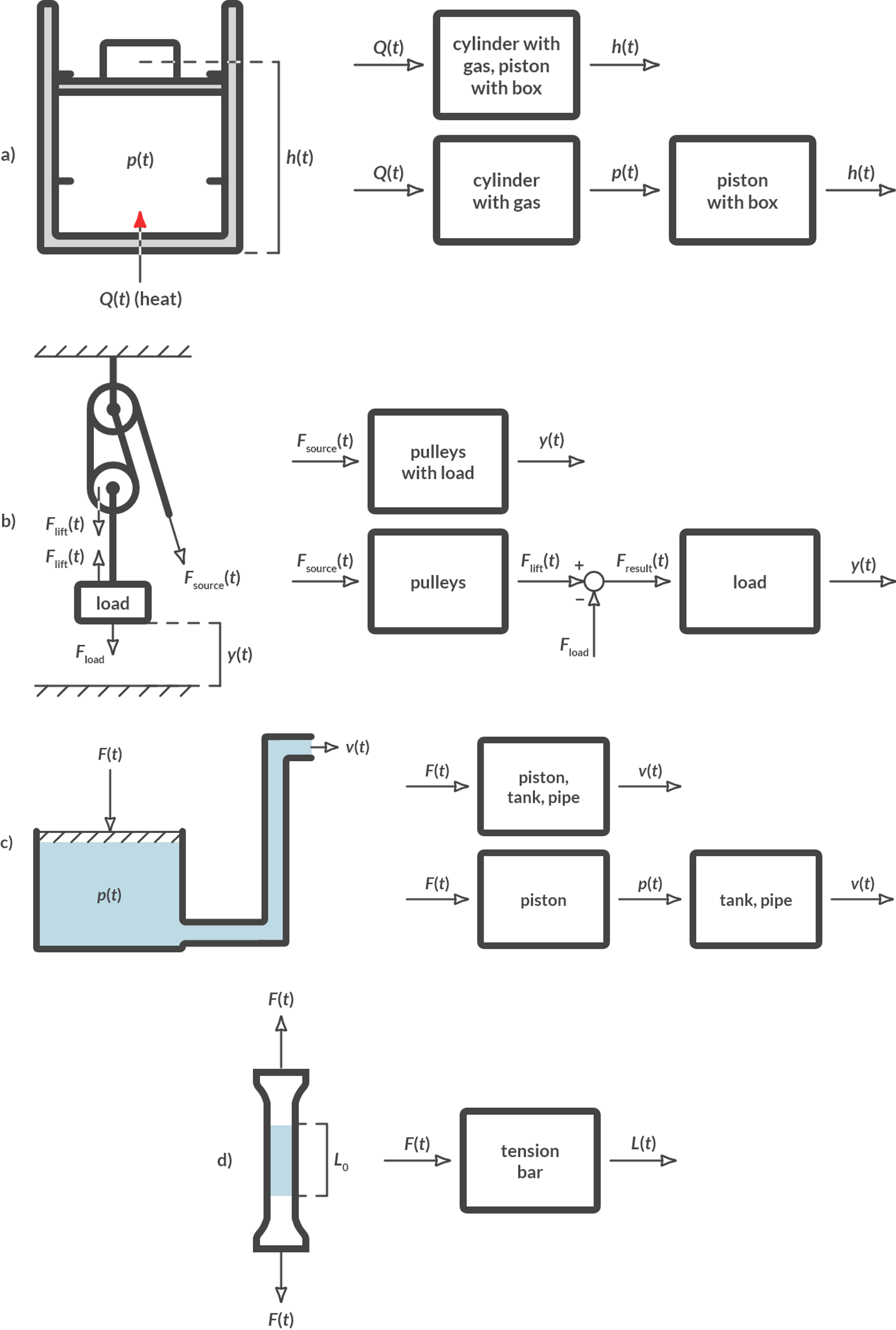
Fig. 6.3 Examples of block diagrams.

The block functions describe the relationship between the input and the output. Fig. 6.3 describes this relationship qualitatively. In Fig. 6.3(b), the block function pulleys describes how the input force results in a lifting force on the mass. To quantitatively describe such a relationship, we use a model of physical reality. For simple systems, that model can be a simple equation. For many systems the relationship is described with differential equations (equations in which in addition to variables also derivatives of those variables occur over time).

Fig. 6.4 shows for two examples of Fig. 6.3 how the relationship between input and output with comparisons can be described

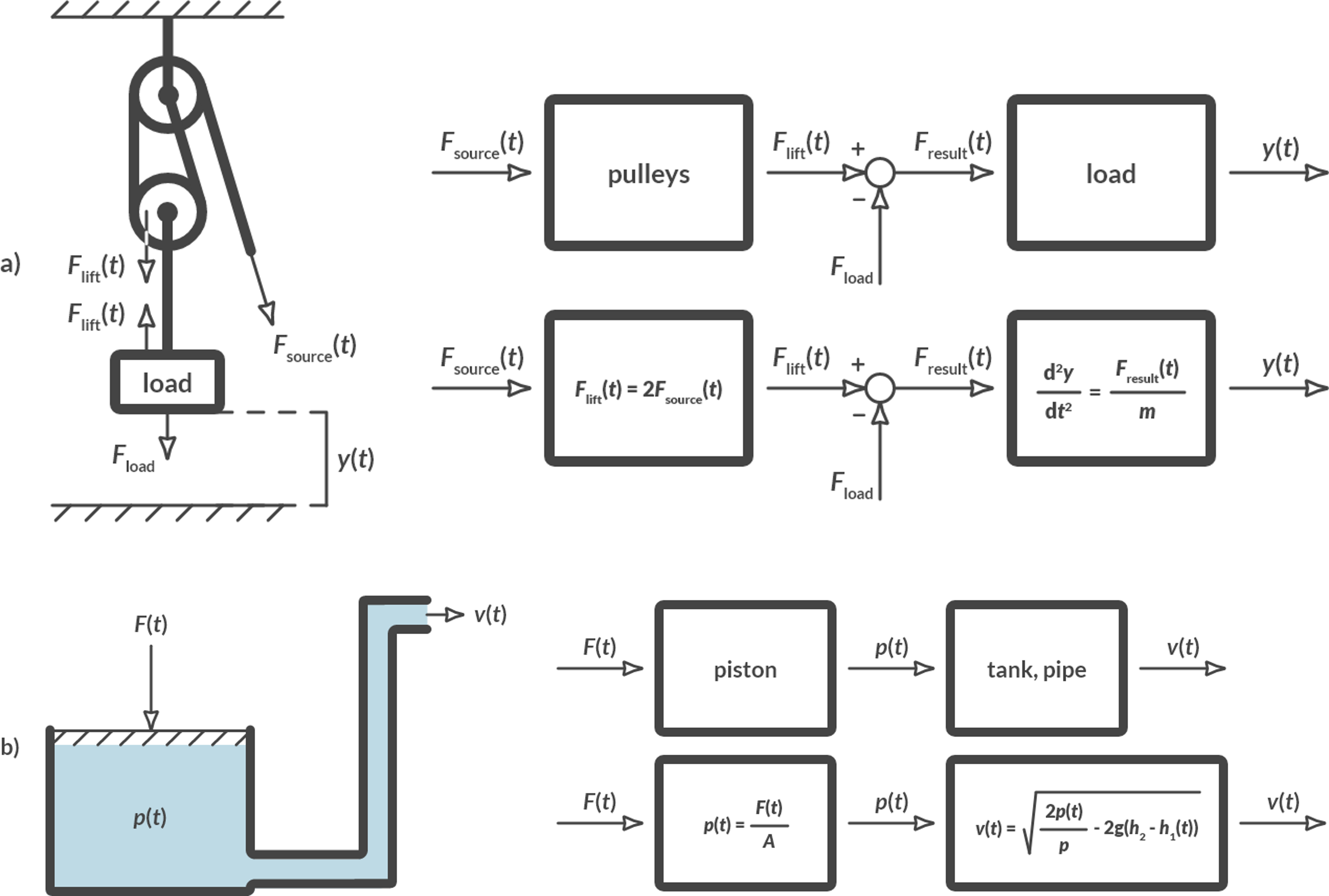
Fig. 6.4 Examples of block diagrams with equations.

We use theory from other disciplines to draw up these equations. In these examples these are dynamics and fluid mechanics, which is discussed in Section 3. Note that the variables are always noted as a function of time \(t\). The other quantities in the equations (the constants) are called parameters.

Quantitative block diagrams

Can you rewrite the block diagrams in Fig. 6.4 into normal (differential) equations? How can these equations be derived?

Solution

The pulleys in Fig. 6.3(a)

• \(F_{\text{lift}}(t) = 2 \cdot F_{\text{source}}(t)\)

• \(F_{\text{res}}(t) = F_{\text{lift}}(t) – F_{\text{load}}\) (\(= F_{\text{lift}}(t) – F_z = F_{\text{lift}}(t) – mg\)), wherein the mass of the lower pulley is neglected.

• \(d^2 \frac{y}{dt^2}=\frac{F_{\text{res}}(t)}{m}\) (\(\frac{d^2 y}{dt^2}\) is the acceleration \(a_y\) in the \(y\)-direction. This is equal to: \(F = m \cdot a\))

We can substitute these three equations together. We then get one equation:

(6.1)\[ \frac{d^2y}{dt^2}=\frac{2\cdot F_{\text{source}}(t)-F_{\text{load}}}{m} \quad \Big[\frac{\textrm{m}}{\textrm{s}^2} \Big]=\frac{[N]}{[kg]} \]

This equation would be the equation of the block function with inputs \(F_{\text{source}}(t)\) and \(F_{\text{load}}\) and output \(y(t)\).

The liquid sprayer in Fig. 6.3(b)

\(p(t) = \frac{F(t)}{A}\\ v(t) = \sqrt{\frac{2}{\rho}-2g(h_2-h_1(t))}\)

The last equation can be deduced from Bernoulli’s law, see again Section 3, where the initial speed \(v_1\) is neglected:

(6.2)\[\begin{split} p_1 + \rho g h_1 + \frac{1}{2} \rho v^2_1 = p_2 + \rho g h_2 + \frac{1}{2} \rho v^2_2 \\ p + p_b +\rho g h_1 = p_b + \rho g h_2 + \frac{1}{2} \rho v^2\\ \frac{1}{2}\rho v^2 = p - \rho g (h_2-h_1)\\ v= \sqrt{\frac{2}{\rho}\frac{F}{A}-2g(h_2-h_1)} \end{split}\]

6.3. The feedback principle

In control technology, we often look at system behavior over time. For example, the position \(y(t)\) of a mass (see Fig. 6.4(a)), or the temperature \(T(t)\) of swimming pool water or the flow rate \(v(t)\) of a liquid sprayer (Fig. 6.4(b)). In the previous section we have seen several examples of open (unregulated) systems. We take a certain input value (for example a constant value) without measuring the output and checking whether we need to adjust the input. If, for example, we consider the system of Fig. 6.4(b), then we see that if \(F(t)\) remained constant, \(v(t)\) would change over time: the vessel empties, so the height \(h_1(t)\) decreases and thus the velocity \(v(t)\) decreases over time. In order to keep the velocity \(v(t)\) constant, we will have to change \(F(t)\) over time, so control it.

In control engineering, the goal is often to let a variable follow a certain course over time. In this introduction we only consider the goal of keeping a variable at a constant value.

6.3.1. Steering versus controlling

We must distinguish here between the concepts of “steering” and “controlling”. With “steering” we offer an open system such an input signal that the output shows a certain (desired) behavior in time. Our knowledge of system behavior makes it possible to make the right choice for this input signal. With “controlling” we proceed differently: we look at the output of the system and if it deviates from the desired course, we will adjust something based on the difference at the input of the system, so that the deviation becomes less. In this way the output is fed back to the input and a “feedback control” is created. When controlling systems, instead of looking at the output, the correct input is selected and offered to the system based on experience (knowledge of system behavior). It will later appear that the principle of (closed) feedback systems offers great advantages over (open) control, but that there are also risks attached to it.

Controlling the liquid sprayer

Consider the liquid sprayer of Fig. 6.4(b). It is desirable to achieve a constant spraying velocity during spraying. The force \(F(t)\) on the piston can be used for this purpose. What does the block diagram of the regulated system look like?

Solution

Fig. 6.5 shows the control loop on the left in a schematic representation of the physical system. The block diagram is shown on the right.

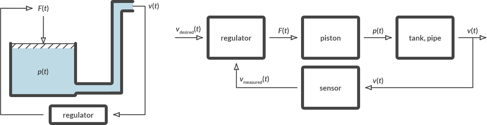
Fig. 6.5 Controlled liquid sprayer.

In practice there are numerous control loops. In general, a control loop looks like this:

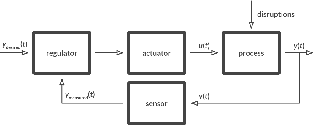
Fig. 6.6 General control loop.

The elements in this general control loop are:

• the process that must be controlled (the system to be controlled),

• the (often unknown) disruptions that affect the process,

• the measuring instrument (sensor) that measures an output of the process,

• the actuator that intervenes in the process

• the control algorithm (the controller) that controls the actuator based on a desired signal \(y_{\textrm{des}}(t)\) and the measured signal \(y_{\text{meas}}(t)\).

Thermostat

How does the control circuit of a thermostat of a living room look like? What do we want to control? How can we arrange? What are the disruptions? Draw a block diagram of the controlled system. Name the components in the control circuit (actuator, sensor, process, disruptions).

Solution

The thermostat ensures that the desired temperature is maintained in a room. The measured variable, the process output \(y(t)\), is the room temperature \(T(t)\) at the location of the sensor. The thermostat can influence the temperature by turning the heating (boiler) up or down. The control variable, the process input \(u(t)\), is the heat \(Q(t)\) supplied.

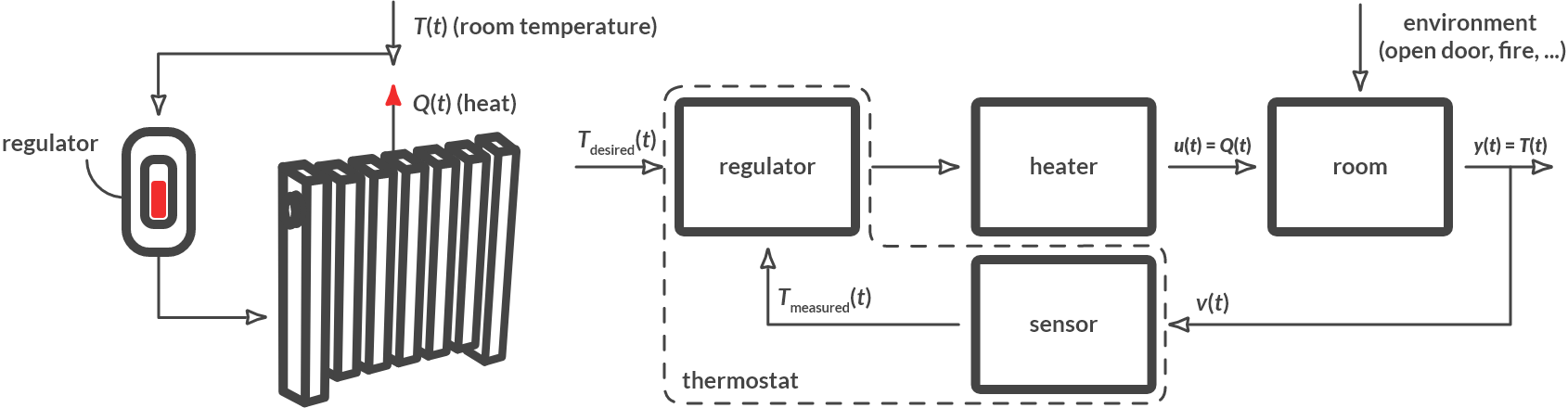
Fig. 6.7 Room temperature control.

Examples of disruptions are the heat losses to the outside (if the outside temperature changes), the opening of the outside door or the lighting of a fire in the fireplace. The thermostat contains both the sensor and the controller.

Other examples of control loops are:

• a driver who wants to continue driving straight on a road,

• the altitude control of an aircraft,

• the speed regulation of a car (cruise control),

• the temperature regulation of the water when you are in the shower.

Note

Can you draw the same kind of control circuit in block diagram notation from those examples?

6.4. Controller design

In the previous section you saw that you can control the dynamic behavior of a process by measuring an output of a process and changing it based on that. But how should you change the input if you have measured the output? Numerous methods have been developed in control engineering. Here we only deal with the most basic method, the so-called proportional control.

First, we define the error. The error \(e(t)\) is the difference in signal between the desired value \(y_{\textrm{des}}(t)\) and the measured value \(y_{\text{meas}}(t)\). With proportional control, we let the input signal of the process depend proportionally on the error. By way of illustration we consider the room temperature control of Example 3. To make a quantitative analysis possible, we replace the qualitative descriptions with a quantitative model. The model of Fig. 6.8 is given.

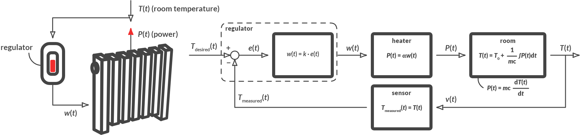
Fig. 6.8 Room temperature control.

In the block diagram we can already see that the controller makes its output signal \(w(t)\) proportionally dependent on the error \(e(t)\), since \(w(t) = k \cdot e(t) = k \cdot (T_{\text{des}}(t) – T_{\text{meas}}(t))\). Herein we call k the gain. That is a nice idea in itself, because:

• If \(T_{\text{meas}}(t)< T_{\text{des}}(t)\), it is too cold. Then \(e(t)> 0\). The controller gives output signal \(w(t)> 0\). The heating supplies a positive power (supplies heat) \(P(t)> 0\). The temperature increases.

• If \(T_{\text{meas}}(t) > T_{\text{des}}(t)\), it is too hot. The controller gives output signal \(w(t) < 0\). The heating produces a negative power (extracts heat) \(P(t) < 0\). The temperature decreases.

• If \(T_{\text{meas}}(t) = T_{\text{des}}(t)\), the temperature is just right. The controller gives output signal \(w(t) = 0\). The heating does not supply power \(P(t) = 0\). The temperature remains unchanged.

We now want to investigate how the temperature changes if we want to reach a temperature of 20 °C, while the initial temperature is 0 °C. For this we have to solve the following equations. Precisely take into account the meaning of all symbols and their units. Be consistent in their unambiguous use!

\[\begin{split} P(t) = \alpha w(t)\\ w(t) = ke(t) = k(T_{\textrm{des}}-T_{\textrm{meas}}(t))\\ T_{\textrm{meas}}(t)=T(t)\\ P(t)=C_p\frac{dT(t)}{dt} \end{split}\]

After elimination of \(P(t), w(t),\) and \(T_{\textrm{meas}}(t)\) this becomes:

(6.3)\[\alpha \cdot k (T_{\textrm{des}}-T(t))= C_p \frac{dT(t)}{dt}\]

The result is a differential equation, which we can rewrite:

(6.4)\[ \frac{dT(t)}{dt} + \frac{k\alpha}{C_p}T(t)= \frac{k\alpha}{C_p}T_{\textrm{des}} \quad \text{or} \quad \dot{T} + \frac{k\alpha}{C_p}T = \frac{k\alpha}{C_p}T_{\textrm{des}} \]

Herein \(\dot{T}\) (pronounced T-dot) is the time derivative of \(T(t)\), or \(\frac{dT(t)}{dt}\). In this introductory course we do not come to the solution of differential equations. That is why we provide the solution of the above equation without derivation. You can check that this solution complies with (6.4) by determining the derivative of (6.5) and entering it in (6.4).

(6.5)\[ T(t)=T_{\textrm{des}}+(T_0-T_{\textrm{des}})e^{-\frac{k\alpha}{C_p}t} \]

Suppose the initial temperature \(T_0 = T(t=0) = T(0) = 0 °C\). Fig. 6.9 shows the temperature trend over time. It is assumed that the heat capacity of the chamber \(C_p\) = 3000 [kJ/K], the heating constant = 1 [-] and the control gain \(k\) = 1000 [W/°C].

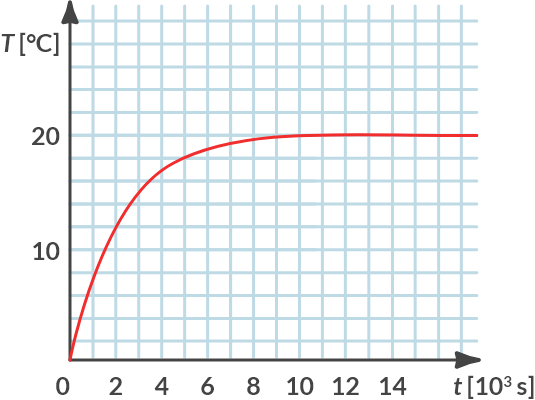
Fig. 6.9 Temperature in time for \(k\) = 1000 [W/°C].

We see that it takes a certain time until the desired temperature of 20 °C is reached (approached). At \(t = 12 \cdot 10^3 \textrm{ s}\) the temperature has risen to \(T = 19.63 \textrm{ °C}\).

By choosing a different control setting for control gain \(k\) we can shorten or extend that time. Increasing the control gain \(k\) shortens the warm-up time. This is shown in Fig. 6.10(a). However, increasing the control gain \(k\) also requires a higher control effort: the heating must then be able to provide a higher power. In Fig. 6.10(b), the power that the heating must provide is plotted against time for different values of \(k\).

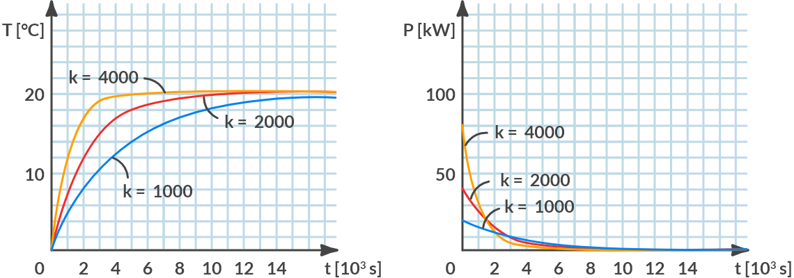
Fig. 6.10 (a) Temperature variation, (b) required power for different control gains.

For \(k = 4000 \textrm{ W/°C}\), the heating must provide a maximum power at \(t = 0\) s of \(80000\) W.

Analysis of room temperature control

Using temperature control, we want to keep the temperature in a room constant. We use the room temperature control model described above. We want to heat the room from 10 °C to 30 °C. For the heating constant, take \(\alpha = 1 [-]\) and for the heat capacity \(C_p = 6000 \textrm{[kJ/K]}\). We can set the room temperature control to three positions, namely \(k = 500 \textrm{W/°C}\), \(k = 1000 \textrm{ W/°C}\) en \(k = 1500 \textrm{ W/°C}\).

1. For each control gain, determine how long it takes for the error to be less than 1 °C.

Solution

1. The regulated temperature as a function of time is given by:

(6.6)\[ T(t) = T_{\textrm{des}} + (T_0-T_{\textrm{des}})e^{-\frac{k\alpha}{C_p}t} \]

If the error must be less than 1 °C, the temperature must be higher than 29 °C and lower than 31 °C. Since the starting temperature is 10 °C, the regulated temperature will rise monotonously. Therefore, the first time the error becomes smaller than 1 °C will occur if the temperature reaches 29 °C.

Solving T(t) = 29 °C gives:

\[\begin{split} T_{\textrm{des}} + (T_0-T_{\textrm{des}})e^{-\frac{k\alpha}{C_p}t} = 29\\ 30 + (10-30)e^{-\frac{k\alpha}{C_p}t} = 29\\ -20e^{-\frac{k\alpha}{C_p}t}=-1\\ \ln(20e^{-\frac{k\alpha}{C_p}t})=\ln(1)\\ \ln e^{-\frac{k\alpha}{C_p}t} = 0 -\ln(20)\\ -\frac{k\alpha}{C_p}t= -\ln(20)\rightarrow t=\frac{C_p}{k\alpha}\ln(20) \end{split}\]

With \(\alpha = 1\), \(C_p = 6000 [\textrm{kJ/K}]\) and \(k = 500 [\textrm{W/°C}]\), \(k = 1000 [\textrm{W/°C}]\) and \(k = 1500 [\textrm{W/°C}]\) t becomes:

(6.7)\[\begin{split} \begin{aligned} k & = 500 [\textrm{W/°C}] & \text{For } t > 35,9 \cdot 10^3 \textrm{[s]} : e(t) < 1 °C \\ k & = 1000 [\textrm{W/°C}] & \text{For } t > 18,0 \cdot 10^3 \textrm{[s]} : e(t) < 1 °C \\ k & = 1500 [\textrm{W/°C}] & \text{For } t > 12,0 \cdot 10^3 \textrm{[s]} : e(t) < 1 °C \end{aligned} \end{split}\]

2. How does the error proceed over time? When is the error nil?

Solution

2. The error changes from a maximum of 20 °C on \(t\) = 0 [s] to 0 °C for \(t \rightarrow \infty\). For larger values of \(k\), the error decreases faster. In Fig. 6.11(a) the error is plotted against time.

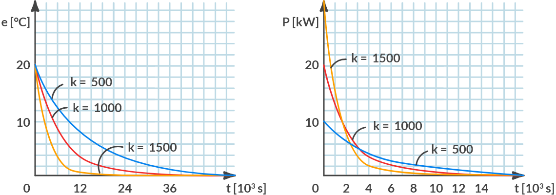
Fig. 6.11 (a) Control error, (b) Control effort (heating capacity) against time.

3. How changes the power that the heating system has to deliver over time? If the heating can supply a maximum of 22 [kW], which control gain(s) is (are) feasible?

Solution

3. The power to be supplied by the heating is proportional to the error:

(6.8)\[ P(t) = \alpha \cdot w(t)= k \cdot \alpha \cdot e(t)= k \cdot \alpha \cdot (T_{\textrm{meas}}(t)-T_{\textrm{des}}) \]

The change in power over time is shown in Fig. 6.11 (b). The maximum power is supplied at \(t\) = 0 [s]. For the different values of k that is equal to:

(6.9)\[\begin{split} \begin{aligned} k & = 500 [\textrm{W/°C}] & P(t=0) = k \cdot \alpha \cdot (T_{\textrm{meas}}(0) - T_{\textrm{des}}) & = 500 [\textrm{W/°C}] \times 20 [° \textrm{C}] & = 10 \textrm{[kW]} \\ k & = 1000 [\textrm{W/°C}] & P(t=0) = k \cdot \alpha \cdot (T_{\textrm{meas}}(0) - T_{\textrm{des}}) & = 1000 [\textrm{W/°C}] \times 20 [° \textrm{C}] & = 20 \textrm{[kW]} \\ k & = 1500 [\textrm{W/°C}] & P(t=0) = k \cdot \alpha \cdot (T_{\textrm{meas}}(0) - T_{\textrm{des}}) & = 1500 [\textrm{W/°C}] \times 20 [° \textrm{C}] & = 30 \textrm{[kW]} \end{aligned}\end{split}\]

If the maximum power of the heating is 22 [kW], only the control positions \(k = 500 [\textrm{W/°C}]\) and \(k = 1000 [\textrm{W/°C}]\) are possible.

6.5. What lies ahead

Before we look further, first something about the history of the profession. The “system and control technology” is a relatively young field. About 60 years ago, the first electronic control schemes were built and insight into the issue of stability through feedback and design rules for single-input and single-output systems were created. Approximately forty years ago, partly due to the developments in aerospace at that time, a mathematical deepening of the field was created that made it possible to design optimum controllers for systems with more inputs and outputs (“multi-variable systems”). In the 1980s much work was done to take model errors into account (robust control and adaptive control), while the last ten years have been dominated by self-learning systems (neural networks), non-linear control and control of hybrid systems (systems with continuous variables and discrete events, such as an operator pressing a button). At the same time there has been a huge development of tools, of which Matlab is the most important. Originating in this field, Matlab is now the most widespread auxiliary tool of the modern engineer. One of the interesting additions to Matlab is Simulink, which makes it easy to model dynamic control systems with block diagrams and then simulate them. The examples from the previous paragraph are very easy to try. With the help of these tools, modeling and control are dealt with in the follow-up courses, first of one-input/one-output systems, and then of multi-variable systems.

Today, in many technical applications, the controller is completely captured in computer code that is executed in real time. Many applications are also known with electronic controllers (circuits with electronic components that provide a filtering effect, e.g. “RC” network). Finally there are the mechanical, hydraulic or pneumatic controllers, although the function of controller and actuator are often combined in one physical device.

An interesting thought is that the relevant considerations for the design of a control system naturally have a lot to do with the design of the process itself (and also which inputs and outputs are useful), as well as the design of the actuator and sensor. The integrated approach to the design of regular mechanical devices is also called “mechatronics”. This will be discussed in detail in later courses.

In the master’s phase, the most important developments in the field as described above are discussed in more detail. Active research topics are robust, non-linear and learning arrangements of mechatronic systems, automotive applications and applications in robotics, biomedical and process engineering systems.

6.6. Problems

For the following exercises use symbols as long as possible and only in the end fill in the values given.

Exercise 6.1 (CD-player control)

The information on a cd is recorded in one long spiral shaped track. For reading this track a laser reading head (Laser Pickup) is used. The reading head can be moved by means of a motor (Tracking Motor). This has been depicted schematically in Fig. 6.12. The other motor, Disc Motor, guarantees that the cd rotates with the correct velocity. The information density (amount of information per mm) on a cd is equal over the entire track. When the reading head is close to the center of the cd, the cd should spin with a larger angular velocity than when the reading head is close to the edge of the cd.

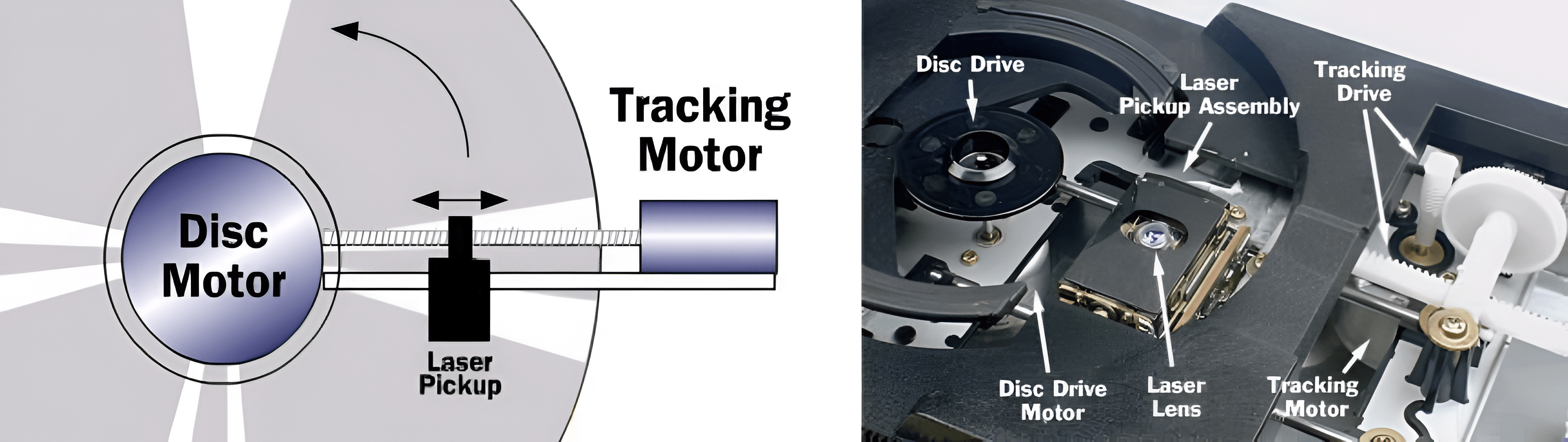
Fig. 6.12 Schematic representation of cd with reading head (left), interior of a cd player (right).

In this exercise we consider the situation where the laser read head is at a constant distance R from the center of the cd. The cd then has to spin with a constant angular velocity. Therefore, we use a feedback control loop, schematically depicted in Fig. 6.13.

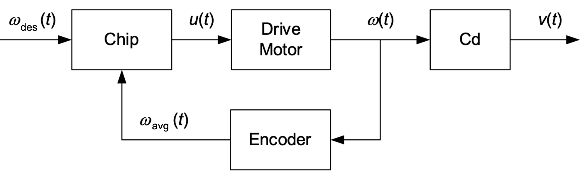
Fig. 6.13 Block diagram of cd-player.

1. What are the (A)ctuator, (S)ensor, and (C)ontroller in the block diagram of Fig. 6.13?

In this control loop the angular velocity of the cd is not measured, only the angular velocity of the motor that makes the cd spin. It is given that the laser reading head is at a radius of R = 40mm from the center of the cd. The desired tangential velocity of the cd is \(v_{\textrm{des}} = 1.20 \textrm{m}/\textrm{s}\). For \(R = 40\) mm this corresponds with a desired angular velocity of the motor \(\omega_{\textrm{des}} = 30\) rad\(/\)s. We assume that the controller has managed to realize this desired angular velocity perfectly.

2. Explain if we can claim with certainty that the tangential velocity of the cd at the reading head is indeed 1.20 \(\textrm{m}/\textrm{s}\).

The following equations are given to describe a part of the system dynamics. The problem parameters are givne in Table 6.1.

(6.10)\[\textrm{Encoder}: \: \omega_{\textrm{avg}} (t) = \omega (t)\]

(6.11)\[\textrm{Motor}: \: J\, \dot{\omega} (t) + b\, \omega (t) = \alpha\, u(t)\]

Table 6.1 Parameters CD dynamics

	Parameters
\(\omega_{\textrm{avg}} (t)\)	The measured angular velocity of the drive motor in [rad\(/\)s].
\(\omega (t)\)	the actual angular velocity of the drive motor in [rad\(/\)s],
\(J\)	the inertia of the motor, cd and suspension in [\(\textrm{Nms}^2/\textrm{rad}^2\)].
\(b\)	the damping (due to friction) in [Nms\(/\)rad].
\(\alpha\)	A constant in [Nm\(/\)A] with \(\alpha > 0\).
\(u(t)\)	The control signal in [A].

For the chip we choose

(6.12)\[u(t) = k(\omega_{\textrm{des}} (t) - \omega_{\textrm{avg}} (t))\]

For the chip we choose the parameters in Table 6.2

Table 6.2 Parameters chip

	Parameters
\(\omega_{\textrm{des}}\)	The desired angular velocity of the drive motor in [rad\(/\)s].
\(k\)	The control gain in [\(As/\)rad].

3. Explain that for k\( > 0\) the chip controller achieves the desired behavior.

4. Reduce by means of elimination\(/\)substitution the set of equations (6.10) - (6.12) to the following differential equation

(6.13)\[ \dot{\omega} (t) + \frac{b + \alpha\, k}{J}\, \omega (t) = \frac{\alpha \, k}{J} \, \omega_{\textrm{des}} (t).\]

We first want to develop a feeling for how the angular velocity evolves over time. We assume a constant desired angular velocity, i.e., \(\omega_{\textrm{des}} (t) = \bar{\omega}\). Furthermore, we assume that the initial angular velocity is \(\omega(0) = 0\) rad/s.

The following solution for the differential equation (6.13) is proposed:

(6.14)\[ \omega (t) = \frac{\alpha \, k}{b + \alpha \, k} \, \bar{\omega}(1-e^{-t/\tau}).\]

5. Show that for \(\tau = \frac{J}{b+\alpha \, k}\) and the above mentioned assumptions this solutions satisfies the differential equation (6.13). Furthermore, show that this solution satisfies the required initial condition.

6. Calculate which angular velocity is achieved for \(t \rightarrow \infty \).

The difference between the desired angular velocity \(\omega_{\textrm{des}} (t) = \bar{\omega}\) and the actual angular velocity \(\omega(t)\) is called the control error \(e(t)\).

7. What can be said about \(b, \alpha\) and \(k\) in relation to the control error \(e(t)\) for \(t \rightarrow \infty\) ?

Exercise 6.2 (Cruise control)

To have a car drive at a constant velocity, many cars are nowadays equipped with cruise control that can be controlled from the steering wheel. In this exercise we want to gain insight in the design of such a system. In Fig. 6.14 a simplified version is given of a block diagram describing a car with cruise control.

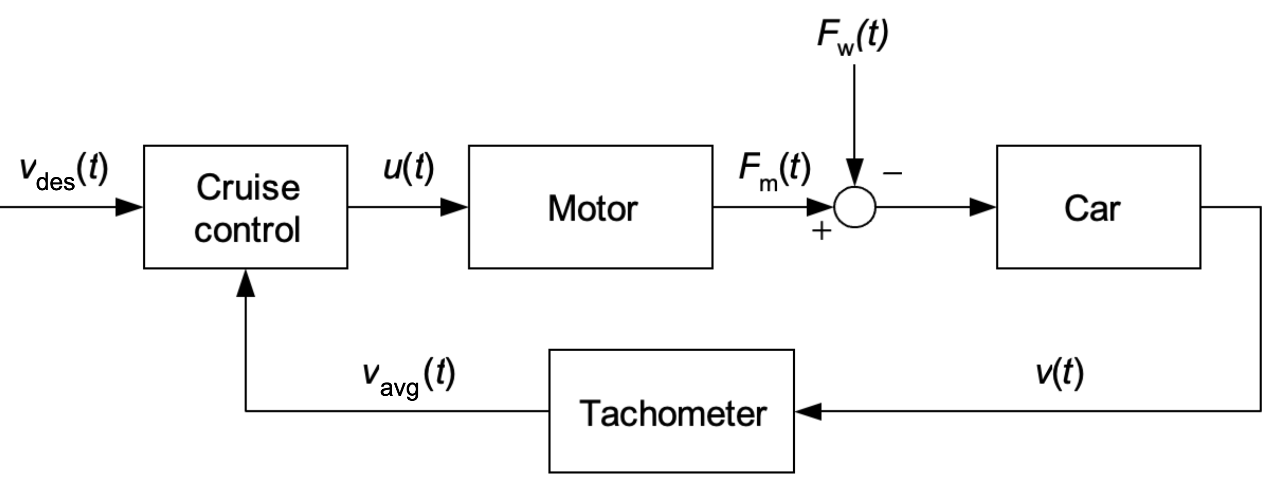
Fig. 6.14 Block diagram of a cruise controlled car.

1. What are the (A)ctuator, (S)ensor, and (C)ontroller in the block diagram of Fig. 6.14?

The equations (6.15)-(6.17) are given to describe a part of the system dynamics.

(6.15)\[\textrm{Tachometer}:\: v_{\textrm{avg}} (t) = v(t)\]

(6.16)\[\textrm{Motor}:\: F_m (t) = \alpha \, u(t)\]

(6.17)\[\textrm{Car}:\: \dot{v}(t) = \frac{F_m (t) - F_w (t)}{m}\]

The dynamics parameters are give in Table 6.3.

Table 6.3 Parameters dynamics

	Parameters
\(v_{\textrm{avg}} (t)\)	The measured velocity of the the car in [m\(/\)s].
\(v (t)\)	The actual velocity of the the car in [m\(/\)s].
\(F_m (t)\)	The motor force in [N].
\(\alpha\)	A constant in [-] with \(\alpha > 0\).
\(u(t)\)	The control signal in [N].
\(F_w\)	The friction force in [N].
\(m\)	the mass of the car in [kg].

2. Deduce by means of Newton’s second law that the dynamics of the car can be described by means of equation (6.17). Also, make a schematic overview of the car with the forces acting on it (according to this model).

For the cruise control we choose

(6.18)\[\textrm{Cruise-control}:\: u (t) = k(v_{\textrm{des}} (t)-v_{\textrm{avg}} (t))\]

The cruise control parameters are give in Table 6.4.

Table 6.4 Parameters cruise-control

	Parameters
\(v_{\textrm{des}} (t)\)	The desired velocity of the the car in [m\(/\)s].
\(k\)	The control gain in [Ns\(/\)m].

3. Explain that for \(k > 0\) the controller achieves the desired behavior. (Check what happens if the car drives too slowly of too fast.)

4. Reduce by means of elimination\(/\)substitution the set of equations (6.15) - (6.18) to the following differential equation

(6.19)\[\dot{v} (t) + \frac{\alpha \, k}{m}\, v(t) = \frac{\alpha \, k}{m}\, v_{\textrm{des}} (t) - \frac{1}{m}\, F_w (t)\]

We now first want to develop some feeling for how the velocity v evolves as a function of time t. Therefore, we make three assumptions:

• Friction is ignored, i.e., \( F_w (t) = 0\) N.

• We assume a constant desired velocity, i.e., \(v_{\textrm{des}} (t) = \bar v\).

• We assume the initial velocity is \(v (0) = 0\) m/s.

(6.20)\[v (t) = \bar{v}(1-e^{-t/\tau})\]

is proposed as a solution to the differential equation (6.19).

5. Show that for \(\tau = \frac{m}{\alpha \, k}\) and the above mentioned assumptions this solution satisfies both the differential equation (6.19) and the initial condition \(v (0) = 0\) m/s (so both!).

6. We consider the situation where a car accelerates from standstill to a desired velocity to \(5\) m/s. Sketch “qualitatively” the evolution of velocity as a function of time (no actual values are required). Indicate in this sketch how the evolution changes in case of:

• A larger value for \(k\).

• A larger value for \(m\).

• A larger value for \(\alpha\).

Exercise 6.3 (Robot localization)

An autonomous robot often needs to load information from a digital map. This digital map represents the robot’s environment in a robot understandable way and allows for performing tasks, such as navigating from \(A\) to \(B\). Before the robot can make use of map information, it needs to compute its position with respect to the elements in this map. This process is called ‘robot localization’. Fig. 6.15 shows a 1D world including a robot and two landmarks whose positions are known from a map. The coordinates of the landmarks are denoted by \(x_{lm1}\) and \(x_{lm2}\). The robot’s position, \(x_r\), is constrained to be: \(x_{lm1}\leq x_r \leq x_{lm2}\). In order to compute the robot position, the robot has a sensor that can be used to measure the distance to each of the two landmarks (in meters):

(6.21)\[z_1 = x_r - x_{lm1},\]

(6.22)\[z_2 = x_{lm2} - x_r,\]

where \(z_i\) is the absolute distance from robot to landmark i, and \(i=1,2\).

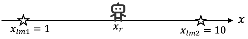
Fig. 6.15 Robot moves on a line. The robot can measure the distance to each of the two landmarks (represented by the stars).

1. The robot receives the following pair of measurements:

• \(z_1 = 4.00\) m

• \(z_2 = 5.00\) m

Compute the robot positioning using these measurements.

In reality, sensor noise leads to imperfect measurements. For example, instead of measuring \(z_1=4.00\) m,\(z_2=5.00\) m, the robot may measure \(z_1=3.95\) m, \(z_2=5.12\) m. In this case, performing robot localization is no longer trivial.

In order to compute the most likely robot position in the presence of sensor noise, we want to find the robot position that ‘best explains’ the measurements. Therefore, the first step is to define a cost function that can later be minimized.

2. The measurement error \(e_i\) is defined by the difference between \(z_i\) and the expected measurement for a given robot position \(x_r\). Derive the expressions for the errors \(e_1\) and \(e_2\). Then, define a cost function \(f(x_r)=e_1^2+e_2^2\).

The cost function allows for computing a cost for each possible robot position, given a pair of measurements. The next step is to find the robot position that best explains the measurements with respect to the cost function.

3. The robot performs two measurements \(z_1=2.2\) m and \(z_2=7.2\) m. Compute the robot position \(x_r\) that minimizes the cost function derived in the previous question.

Tip

this includes computing the derivative of the cost function and setting it to zero.

In reality, a robot may have multiple sensors with different characteristics. The cost function allows for incorporating measurements with different accuracies, e.g., by changing it into a weighted sum of squared error terms.

4. Imagine the measurement \(z_1\) in the previous question was performed with a sensor that is twice as accurate as the sensor used for performing measurement \(z_2\). Use weights in the cost function to account for this difference in measurement accuracy. How will the new cost function look like?

5. What robot position minimizes the new cost function? Compare this robot position with the position computed in question \(3\) and explain the difference.

In this exercise, the cost function was relatively compact and the answer could be computed analytically. In a \(3\)D environment with more landmarks and a more complicated cost function, a similar method can be used for robot localization or even for creating a digital map. In these more complex scenarios, numerical methods are usually employed to find the parameters that minimize a given cost function.

Exercise 6.4 (Drone Control 1)

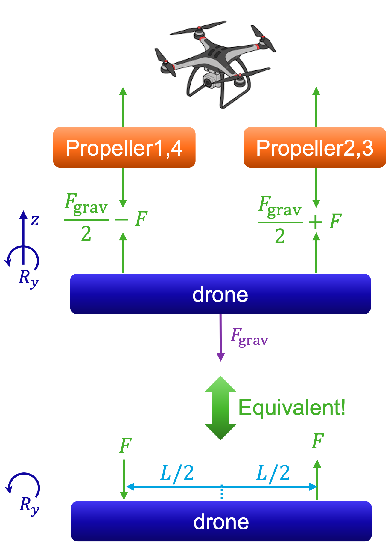
Fig. 6.16 Simplified hover model for a quadcopter in a lateral gust: propeller pairs (1,4) and (2,3) produce \(F_{p1}+F_{p4}=F_{\mathrm{grav}}/2 - F\) and \(F_{p2}+F_{p3}=F_{\mathrm{grav}}/2 + F\), keeping net \(z\)-force and \(R_z\) torque zero; the equivalent two-lift forces, spaced \(L/2\), generate roll about \(R_y\).

In Section 1 of this course, we studied the conditions to let a four-propeller drone hover at rest in the air. In this section, we will investigate how this drone can keep hovering while wind is disturbing its position. The model of the four-propellor drone can be seen in Fig. 6.16.

First, we simplify the four-propeller drone situation by using the following assumptions:

• \(T_{\mathrm{prop}1}=-T_{\mathrm{prop}4}\)

• \(T_{\mathrm{prop}2}=-T_{\mathrm{prop}3}\)

• \(F_{\mathrm{prop}1}+F_{\mathrm{prop}4}=\dfrac{F_{\mathrm{grav}}}{2}-F\)

• \(F_{\mathrm{prop}2}+F_{\mathrm{prop}3}=\dfrac{F_{\mathrm{grav}}}{2}+F\)

1. Check that the sum of z-forces and sum of Rz-torques are indeed zero.

Under these assumptions, the drone will never fall out of the sky (sum of \(\textrm{z-forces} = 0\)), and the drone will never spin around the its z-axis (\(R_z-\textrm{torques} = 0\)).

Because of the assumptions, the drone schematics can be simplified to the bottom schematic in Fig. 6.16. Note that we removed the \(z\) and \(R_z\) axes indication. Instead, in the following questions, we will focus on a new rotation axis: \(R_y\).

Fig. 6.17 Roll about \(R_y\) from differential lift: two upward forces \(F\) applied at \(\pm L/2\) generate a tilt \(\theta\) of the drone.

In Fig. 6.17 it can be seen that the drone can rotate by \(\theta\,\) [rad] around the \(R_y\)-axis. Based on Newton’s second law (see Section 5):

2. Complete the right-hand side of the following relation

   \[I_y \cdot \ddot{\theta} = \sum T_y,\]

   where \(I_y\) [Nms\(^2\)/rad\(^2\)] is the rotational inertia of the drone.

The desired angle of the drone is given by \(\theta_d=0\), a sensor in the drone can measure the actual angle \(\theta\) of the drone, and a feedback controller is present to steer the true angle \(\theta\) towards \(\theta_d\). Given this information, complete the [⋅] parts of the control scheme below in Fig. 6.18.

Fig. 6.18 Closed-loop attitude control: reference \(\theta_d=0\) forms error \(e(t)\) to the controller, producing \(F(t)\); actuators yield \(F_{\text{true}}(t)\) to the drone, whose dynamics output \(\theta_{\text{true}}(t)\); the sensor measures \(\theta(t)\) for feedback.

To avoid making this exercise an MSc project, let us introduce a final simplification: \(F_{\textrm{true}}(t) = F(t)\), i.e., the propellers generate exactly the force we ask for, and \(\theta_{\textrm{meas}}(t) = \theta(t)\), i.e., the sensor measures the actual rotation exactly. This leads to the following simplified control scheme visible in Fig. 6.19 below.

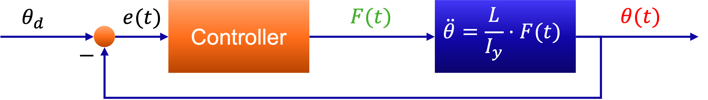
Fig. 6.19 Simplified negative-feedback roll loop: reference \(\theta_d\) generates error \(e(t)\), the controller outputs \(F(t)\), the drone dynamics \(\ddot{\theta}=\tfrac{L}{I_y}F(t)\) yield \(\theta(t)\), which is fed back to close the loop.

After all the assumptions, dynamic modeling, and simplifications, we are finally ready to study the control challenge. Let the controller be a P-controller:

\[ F(t) = k_P \cdot e(t). \]

3. Verify that the closed loop relation \(\theta_d \to \theta(t)\) can be formulated as:

\[ \ddot{\theta}(t)+\frac{L}{I_y}\,k_P\,\theta(t)=\frac{L}{I_y}\,k_P\,\theta_d=0. \]

4. Given this equation, how does the P-controller change the original open loop drone dynamics?

5. What is the eigen frequency of this closed loop system?

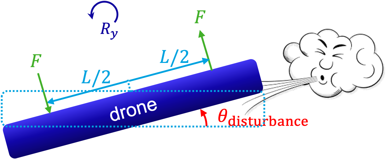
Fig. 6.20 Schematic of the wind gust disturbance where a lateral gust imposes an initial tilt \(\theta_{\text{disturbance}}\); equal lift forces \(F\) applied at \(\pm L/2\) about \(R_y\) produce a restoring roll response.

Consider a wind gust that pushes against the drone as can be seen in Fig. 6.20, giving it an angle \(\theta(0)=\theta_{\textrm{disturbance}}\).

6. Based on what you have learned in Section 5, sketch how \(\theta(t)\) will behave over time for both relatively small and large \(k_P\).

7. Does this P-controller give us the desired behavior \(\theta(t)\to 0\) [rad] over time?

To improve the behavior of the closed loop system, we upgrade our controller to a PD-controller:

\[ F(t)=k_P\bigl(\theta_d-\theta(t)\bigr)+k_D\bigl(\dot{\theta}_d-\dot{\theta}(t)\bigr), \]

with \(\dot{\theta}_d=0\) [rad/s].

8. Verify that the closed loop is now given by

\[ \ddot{\theta}(t)+\frac{L}{I_y}\,k_D\,\dot{\theta}(t)+\frac{L}{I_y}\,k_P\,\theta(t) =\frac{L}{I_y}\,k_P\,\theta_d+\frac{L}{I_y}\,k_D\,\dot{\theta}_d=0. \]

9. How can we physically interpret the \(k_D\) part of the closed loop? Sketch how \(\theta(t)\) will behave over time for both relatively small and large \(k_D\). Can the drone recover from the wind gust disturbance?

Tip

If you look at an airplane while it has commenced the landing procedure, you can see well-damped tilt corrections of the plane while it corrects for wind disturbances: very likely, you then see a PD-like controller in action.

Exercise 6.5 (Drone Control 2)

Fig. 6.21 Simplified hover model for a quadcopter in a lateral gust: propeller pairs (1,4) and (2,3) produce \(F_{p1}+F_{p4}=F_{\mathrm{grav}}/2 - F\) and \(F_{p2}+F_{p3}=F_{\mathrm{grav}}/2 + F\), keeping net \(z\)-force and \(R_z\) torque zero; the equivalent two-lift forces, spaced \(L/2\), generate roll about \(R_y\).

In Section 1 of this course, we studied the conditions to let a four-propeller drone hover at rest in the air. In this section, we will investigate how this drone can keep hovering while wind is disturbing its position. The model of the four-propellor drone can be seen in Fig. 6.21.

As in Exercise 6.4, the lifting force \(F\) to make the drone rotating mide-air is generated by the rotating 4 propellers applying to them torques \(T_{\textrm{prop1}}\), \(T_{\textrm{prop2}}\), \(T_{\textrm{prop3}}\) and T\(_{\textrm{prop4}}\).

First, we simplify the four-propeller drone situation by using the following assumptions:

• \(T_{\mathrm{prop}1}=-T_{\mathrm{prop}4}\)

• \(T_{\mathrm{prop}2}=-T_{\mathrm{prop}3}\)

• \(F_{\mathrm{prop}1}+F_{\mathrm{prop}4}=\dfrac{F_{\mathrm{grav}}}{2}-F\)

• \(F_{\mathrm{prop}2}+F_{\mathrm{prop}3}=\dfrac{F_{\mathrm{grav}}}{2}+F\)

1. Draw the free-body diagram for the drone and the propellers and verify that the drone can hover at rest with this configuration.

2. What conditions must the sum of forces along the z-axis and the sum of torques around the z-axis satisfy for the drone to hover at rest?

Because of the assumptions, the free body diagram of the drone can be simplified to the figure on the bottom left of Fig. 6.21. Note that we removed the \(z\) and \(R_z\) axes indication. Instead, in the following questions, we will focus on a new rotation axis: \(R_y\).

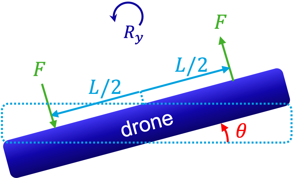
Fig. 6.22 Roll about \(R_y\) from differential lift: two upward forces \(F\) applied at \(\pm L/2\) generate a tilt \(\theta\) of the drone.

In Fig. 6.22 it can be seen that the drone can rotate by \(\theta\,\) [rad] around the \(R_y\)-axis. Based on Newton’s second law (see Section 5):

3. Complete the right-hand side of the following relation

   \[I_y \cdot \ddot{\theta} = \sum T_y,\]

   where \(I_y\) [Nms\(^2\)/rad\(^2\)] is the rotational inertia of the drone.

Without control, the drone would start rotating around the y-axis. To avoid rotation around the y-axis, we need to control our system and keep the actual angle \(\theta_{\text{true}}\) of the drone at the desired value

\[ \theta_d = 0 \ \text{(no rotation)}. \]

We use a feedback control to drive the true angle \(\theta_{\text{true}}\) towards \(\theta_d\). A sensor in the drone can measure the actual angle of the drone.

4. Given this information, complete the \([\cdot]\) parts of the control scheme below in Fig. 6.23.

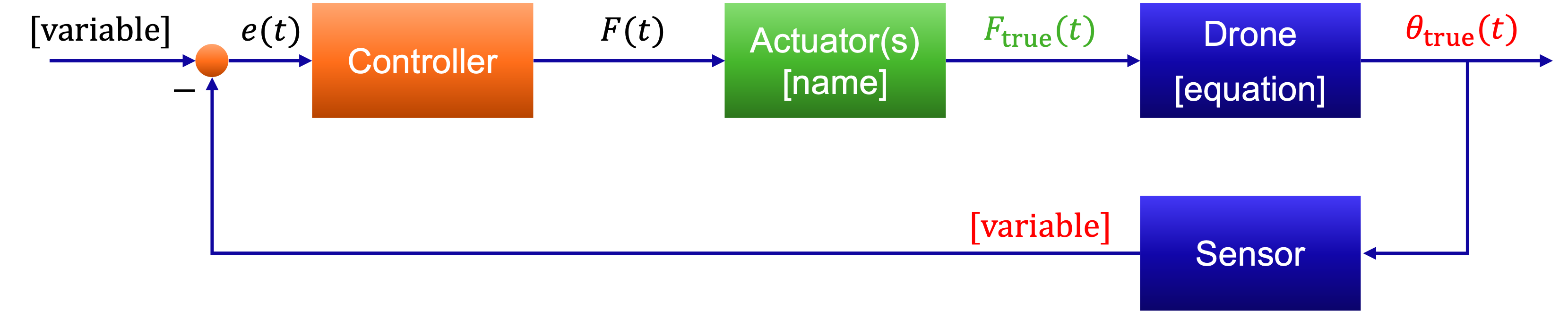
Fig. 6.23 Schematic of a feedback attitude loop, reference input (variable) is compared to the measured angle to form \(e(t)\); the controller outputs \(F(t)\), actuators produce \(F_{\text{true}}(t)\), the drone dynamics map this to \(\theta_{\text{true}}(t)\), and the sensor feeds the measured variable back to the summing junction.

To avoid making this exercise an MSc project, introduce a final simplification:

\[ F_{\text{true}}(t)=F(t), \qquad \theta_{\text{measured}}(t)=\theta(t). \]

The sensor thus measure the actual rotation exactly. This leads to the following simplified control scheme below in Fig. 6.24

Fig. 6.24 Simplified negative-feedback roll loop: reference \(\theta_d\) generates error \(e(t)\), the controller outputs \(F(t)\), the drone dynamics \(\ddot{\theta}=\tfrac{L}{I_y}F(t)\) yield \(\theta(t)\), which is fed back to close the loop.

After all assumptions, dynamic modeling, and simplifications, study the control challenge with a P-controller:

\[ F(t)=k_P \cdot e(t). \]

5. Verify that the closed-loop relation \(\theta_d \to \theta(t)\) can be written as

\[ I_y\,\ddot{\theta}(t)+L\,k_P\,\theta(t)=L\,k_P\,\theta_d=0. \]

6. Given this equation, how can the gain \(k_P\) be physically interpreted?

7. How does the P-controller change the original open-loop drone dynamics?

8. What is the eigenfrequency of this closed-loop system?

Fig. 6.25 Schematic of the wind gust disturbance where a lateral gust imposes an initial tilt \(\theta_{\text{disturbance}}\); equal lift forces \(F\) applied at \(\pm L/2\) about \(R_y\) produce a restoring roll response.

Consider a wind gust that pushes against the drone as can be seen in Fig. 6.25, giving it an angle \(\theta(0)=\theta_{\textrm{disturbance}}\).

9. Based on what you have learned in Section 5, sketch how \(\theta(t)\) will behave over time for both relatively small and large \(k_P\).

10. Does this P-controller give us the desired behavior \(\theta(t)\to 0\) [rad] over time?

To improve the behavior of the closed loop system, we upgrade our controller to a PD-controller:

\[ F(t)=k_P\bigl(\theta_d-\theta(t)\bigr)+k_D\bigl(\dot{\theta}_d-\dot{\theta}(t)\bigr), \]

with \(\dot{\theta}_d=0\) [rad/s].

11. Verify that the closed loop is now given by

\[ I_y\,\ddot{\theta}(t)+L\,k_D\,\dot{\theta}(t)+L\,k_P\,\theta(t) = L\,k_P\,\theta_d + L\,k_D\,\dot{\theta}_d = 0. \]

12. How can we physically interpret the \(k_D\) part of the closed loop?

13. Sketch how \(\theta(t)\) will behave over time for both relatively small and large \(k_D\). Can the drone recover from the wind gust disturbance?