3. Flow machines#
3.1. Introduction#
The number of devices and processes in which flow and/or heat play a major role during the design is endless, see Fig. 3.1 for a few examples. In this chapter we first look at flow machines, where heat does not yet play a role, in the next chapter heat is also discussed. The most important role of flow machines is to convert kinetic or potential energy in the flow into mechanical energy (e.g. wind turbines) or vice versa (e.g. liquid pump).
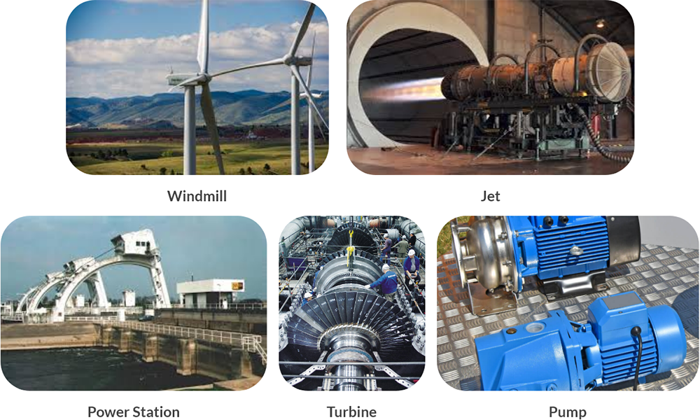
Fig. 3.1 Examples of process equipment used in industry.#
In this chapter you will become acquainted with the principles of fluid mechanics, namely with the different types of flow, the Bernoulli law and pressure losses in pipes.
3.2. Fluids in motion#
3.2.1. Different types of flow#
Flows in a gas or in a liquid are often described with the help of streamlines. Streamlines show how the gas or liquid particles move. Now consider the flow through a pipe section. If we neglect friction, the speed of all particles on line \(I\) (perpendicular to the streamline) is the same. We call this flow laminar frictionless flow (Fig. 3.2(a)).
Note
In English, the flowing medium is referred to as fluid, regardless of whether it is a gas or a liquid.
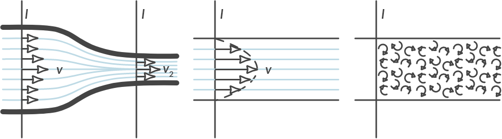
Fig. 3.2 (a) laminar frictionless, (b) laminar, (c) turbulent flow.#
When we consider friction, the situation changes. The velocity of the particles on the wall of the pipe is zero and maximum in the middle. In a pipe with a circular cross-section, the velocity runs parabolic from the center with radius \(r\). We call this flow laminar flow (Fig. 3.2(b)).
If the velocity of the fluid becomes too high, the fluid elements no longer follow a straight line. Vortices and fluctuations of the flow over time arise. There is turbulent flow, something you also notice in an airplane.
3.2.2. Viscosity#
In reality there is always friction. The more viscous the liquid, the more friction. The viscosity \(\eta\) of a liquid is a measure of the resistance that a liquid gives to movement. In Fig. 3.3 you can see two parallel plates, the upper one moving at a speed \(v\) and the lower one being stationary. There is a liquid between the plates. Because the liquid with viscosity \(\eta\) is viscous, a force \(F\) is required to move the upper plate at a constant speed.
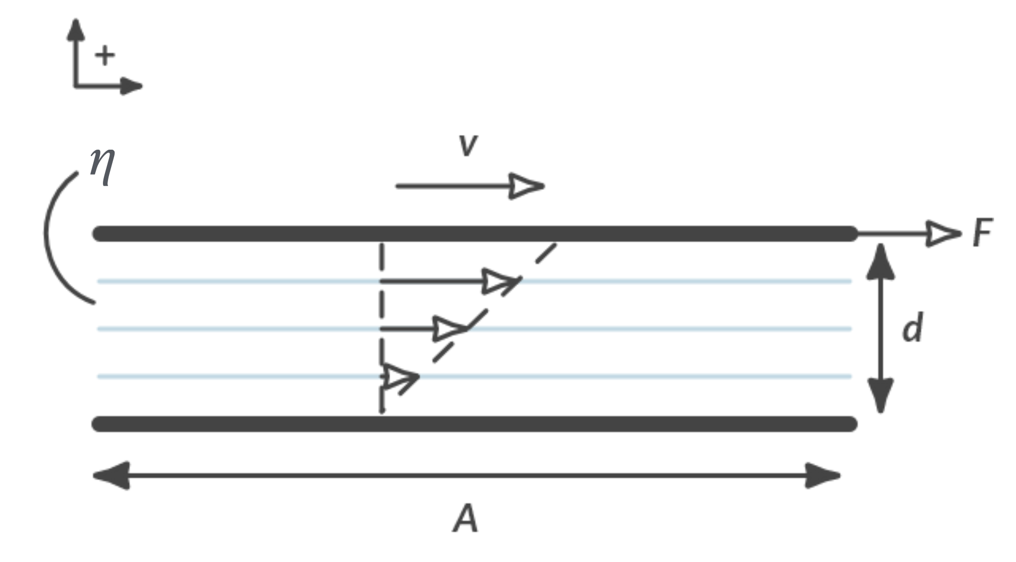
Fig. 3.3 Shear flow in a rheometer to measure viscosity \(\eta\).#
The force \(F\) required depends on the size of the contact surface \(A\), the speed \(v\) of the upper plate, the viscosity \(\eta\) of the liquid and the thickness \(d\) of the liquid layer. As long as the liquid flow is laminar
applies, with \(F\) the necessary force in \([\textrm{N}]\). \(A\) the contact surface in \([\textrm{m}^2]\), \(v\) the velocity of the upper plate [m/s], \(d\) the thickness of the fluid layer in [m] and \(\eta\) the viscosity of the liquid in [Pa·s].
The velocity of the liquid at the upper plate is \(v\), on the lower plate the liquid is stationary. The derivative of speed \(v\) to the position \(y\) is also referred to as the velocity-gradient.
If the ratio between the force \(F\) and \( \displaystyle \frac{v}{d}\) is constant for any \(v\) or \(d\), then we speak of Newtonian behavior and the viscosity \(\eta\) is constant. This is almost always assumed unless we are dealing with complex liquids. Unlike simple fluids that follow Newton’s law of viscosity (where the viscosity is constant regardless of the applied shear rate), complex fluids often exhibit non-Newtonian behavior. This means their viscosity can change depending on the rate of deformation or stress applied to them:
Shear-Thinning: Viscosity decreases with increasing shear rate (e.g., ketchup, paint).
Shear-Thickening: Viscosity increases with increasing shear rate (e.g., cornstarch in water, certain polymers).
Thixotropy: Viscosity decreases over time under constant shear, and recovers when the shear is removed.
Complex fluids also can exhibit both viscous (fluid-like) and elastic (solid-like) responses. This is called viscoelasticity. When subjected to stress, they may temporarily deform and then return to their original shape, similar to how a rubber band behaves.
3.2.3. Continuity equation#
The mass flow \(\dot{m}\) is the mass of water that passes through a cross section per second.
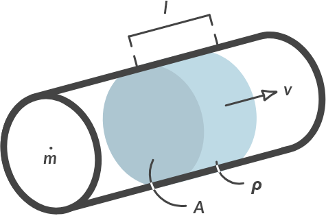
Fig. 3.4 Mass that crosses a section per second.#
applies to the mass flow in Fig. 3.4. In which \(\dot{m}\) (pronounced “m-dot” or fluxie m) is the mass flow in [kg/s], \(\rho\) the density of the flowing medium in \([\textrm{kg/m}^3]\), \(A\) is the cross-section of the pipe in \([\textrm{m}^2]\) and \(v\) the flow speed in [m/s]. It is assumed that \(\rho\) (incompressible, therefore non-compressible, liquid) and \(A\) (non-deformable pipe) are constant. The volume flow \(\Phi_v = A \cdot v\) \([m^3/s]\) indicates the displaced volume of liquid.
If we define a control volume in a liquid, the principle of preservation of mass applies to that control volume: no mass accumulates, and no mass disappears. This means that the mass inflow must be equal to the mass outflow.
T-piece
Below you can see the top view of a horizontally located T-piece. Determine the outgoing flow rates as a function of the incoming flow rates: Given: \(A_2 = A_3 = 0.5 \cdot A_1\)
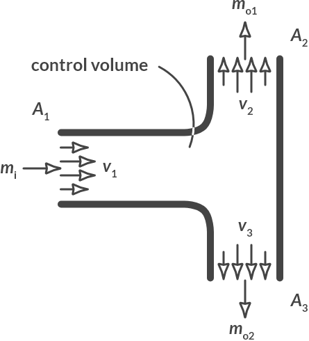
Fig. 3.5 T-piece with incoming and outgoing mass flows.#
From conservation of mass, with i=in and o=out follows:
If we assume for this equation that \(v_2 = v_3\) then \(v_2 = v_3 = v_1\).
3.2.4. Bernoulli’s prinicple#
If you open the door in a flying plane, you will be sucked outside. If you blow past a sheet of paper, the sheet moves to the side you are blowing past (try it!). These phenomena can be explained by Bernoulli’s principle.
Daniel Bernoulli (1700-1782) [1]
Daniel Bernoulli (8 February [O.S. 29 January] 1700 – 27 March 1782) was a Swiss mathematician and physicist and was one of the many prominent mathematicians in the Bernoulli family from Basel. He is particularly remembered for his applications of mathematics to mechanics, especially fluid mechanics, and for his pioneering work in probability and statistics. His name is commemorated in the Bernoulli’s principle, a particular example of the conservation of energy, which describes the mathematics of the mechanism underlying the operation of two important technologies of the 20th century: the carburetor and the aeroplane wing.
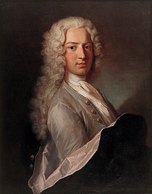
Fig. 3.6 Portrait of Daniel Bernoulli (c. 1720-1725).#
When a liquid is at rest, the hydrostatic pressure \(p\) is determined by the height of the liquid column. When the fluid is in motion, there is also dynamic pressure. Bernoulli’s principle describes how the pressure that a liquid exerts on its environment not only depends on the height of the liquid, but also on the velocity of the flow.
Bernoulli’s principle can be derived by applying the law of conservation of energy (\(\Delta W = \text{ potential energy } \Delta E_p + \text{ kinetic energy } \Delta E_k\)) to a mass element in the liquid. You do not need to be able to reproduce this derivation within the framework of this course. It is advisable to study this for understanding.
A mass element in a stationary flow moves over a streamline. We look at one such mass element at two moments, at \(t = t_0\) and at \(t = t_0 + \Delta t\). The velocity of the mass particle increases because the cross section decreases (continuity equation). This change in velocity is also related to a pressure difference.
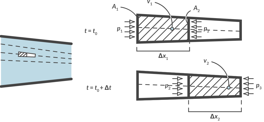
Fig. 3.7 (a) Top view of horizontal flow with increasing speed, (b) mass particle considered in detail.#
Applying the law of conservation of energy to a horizontal flow with increasing velocity as in Fig. 3.7 gives:
The change in velocity of the mass particle is also accompanied by a change in shape of the mass particle. Its diameter becomes smaller, and its length becomes larger, but its mass remains the same. If its density remains the same (and we assume that for liquids), its volume will remain the same. For the volumes we can write:
The work of the pressure equals the force times the distance traveled. At \(t = t_0\) a pressure \(p_1\) acts on the left side of the mass particle and a pressure \(p_2\) on the right side. At \(t = t_0 + \Delta t\) there is pressure \(p_2\) on the left of the particle and \(p_3\) on the right. We assume that the pressure difference over the particle remains constant for a while. (For a small displacement that is allowed.)
The conservation of energy from (3.4) then becomes:
With equation (3.5) and by dividing left and right by \(v\) we finally get:
Equation (3.9) is Bernoulli’s principle, if there is no difference in height in the flow. To now also take into account the effect of height differences, we do the same derivation for a vertical flow.
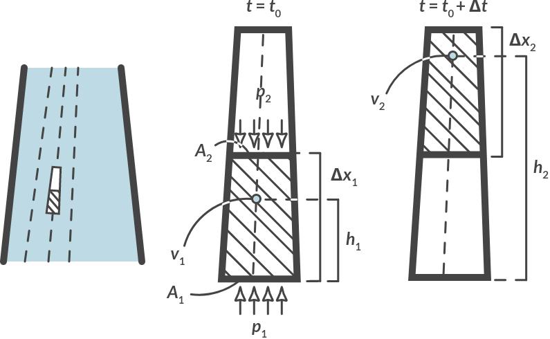
Fig. 3.8 (a) Front view of a vertical flow with increasing speed, (b) mass particle considered in detail.#
In addition to a change in kinetic energy, a change in potential energy also plays a role. Applying the conservation of energy now gives:
With equation (9.4) and by dividing left and right by \(v\) we finally get:
Tip
This result is known as Bernoulli’s Principle:
on one streamline.
All terms have the unit [Nm\(^{-2}] = \textrm{[Pa]}\).
The term \(p\) is the static pressure relative to the environment (pump, air pressure and liquid column pressure).
The terms \(\rho gh\) represent the potential energy of a liquid at height \(h\).
Pay attention! this is not the height of the liquid column, but the height of the streamline.
The term \(\frac{1}{2} ρ v^2\) expresses the kinetic energy of a fluid with a speed \(v\). This term is also called the dynamic pressure.
This is the complete principle of Bernoulli and only applies to one streamline within stationary flow.
Draining barrel
With which velocity does the barrel drain?
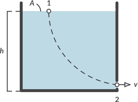
Fig. 3.9 Draining barrel.#
We choose the points 1 and 2 on a streamline. The following applies
\(p_1 = p_2 = p_{\text{atmosphere}}\)
\(h_1 = h, h_2 = 0\)
\(v_1 ≈ 0, v_2 = v\)
Applying the Bernoulli law gives:
Note
With a frictionless free fall from height \(h\) of a mass \(m\), the same relationship applies. Try to deduce this. Note that the size of the falling mass does not play a role in the value of that final velocity.
Pipe with height difference
How much force is needed to operate a sprinkler system at a height of 4 meters at a speed of 5 \(\textrm{m/s}\)? Use \(A_1 = 100\ \textrm{mm}^2, A_2 = 1\ \textrm{mm}^2\).
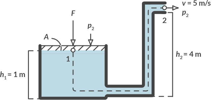
Fig. 3.10 Sprinkler system.#
Solution
We choose points 1 and 2 on a streamline. If the outflow opening is small enough, a mass particle at point 1 must pass point 2. The following applies:
\(p_1 = F/A + p_{\text{atmosphere}}, p_2 = p_{\text{atmosphere}}\)
\(h_1 = 1\ \textrm{m}, h_2 = 4\ \textrm{m}\)
\(v_2 = 5\ \textrm{m/s}, v_1 = \dfrac{v_2 A_2}{A_1} = 0.05\ \textrm{m/s}\) as result of continuity equation
Applying Bernoulli’s principle gives:
Context: a weight of 0.43 kg on a 1 \(\times\) 1 cm piston can pump water up 3 meters an realize a speed of 5 m/s trough a pipe of 1 \(\times\) 1 mm, at least if there is no friction in the pipe.
Pipe with height difference (continued)
It is insightful to choose some other points on the streamline of points 1 and 2. Below you see points 3 and 4 on the same streamline.
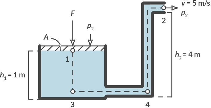
Fig. 3.11 Different points on the same streamline.#
For points 1, 2, 3 and 4 the following applies (with \(\frac{F}{A} = 4.19 \cdot 103 \, \textrm{Pa}\)):
In point 1 |
In point 3 |
In point 4 |
In point 2 |
|
|---|---|---|---|---|
\(p\) |
\( F/A + p_b\) |
\( F/A + p_b + \rho g \cdot 1\) |
\( p_b + \rho g \cdot 4\) |
\( p_b\) |
\(\rho g h\) |
\( \rho g \cdot 1\) |
\( 0 \) |
\( 0 \) |
\( \rho g \cdot 5\) |
\(0.5 \rho V^2 \) |
\( 0.5 \rho \cdot 0.05^2\) |
\( 0.5 \rho \cdot 0.05^2\) |
\( 0.5 \rho \cdot 5^2\) |
\( 0.5 \rho \cdot 5^2\) |
\(\Sigma\) |
\( p_b + 51.74\, \textrm{kPA}\) |
\( p_b + 51.74\, \textrm{kPA}\) |
\( p_b + 51.74\, \textrm{kPA}\) |
\( p_b + 51.74\, \textrm{kPA}\) |
You see that the sum of the three terms (static pressure, potential energy and kinetic energy per volume element) is the same in every point! It is advisable though to choose your points smartly (point 4 is not such an easy choice!).
3.3. Pressure loss in pipes#
We have already seen in Section 3.2 that flowing fluid experiences a frictional force. If we pump a liquid through a pipe, an extra pressure is needed to overcome this wall friction. We say that the frictional force leads to a pressure loss in the pipe. The pressure loss due to wall friction is generally dependent on three factors:
the liquid velocity (and therefore the flow rate and the diameter of the pipe),
the surface condition (roughness) of the inner wall and
the fluid properties such as the density and viscosity of the fluid.
It is common to relate the pressure drop to the average velocity \(v\) of the flow with the Darcy friction factor \(f\):
with:
\(\Delta p\) the pressure loss in the pipe in [Pa],
\(L\) the length of the pipe in [m],
\(D\) the diameter of the pipe in [m],
\(\rho\) the density of the liquid in \([\textrm{kg}/\textrm{m}^3]\),
\(v\) the average (bulk) speed of the flow in [m/s] and
\(f\) de Darcy friction factor [-].
Henry Darcy (1803 - 1858) [2]
Henry Philibert Gaspard Darcy (10 June 1803 – 3 January 1858) was a French engineer who made several important contributions to hydraulics, including Darcy’s law for flow in porous media.
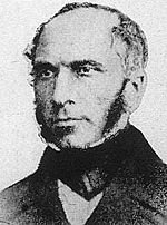
Fig. 3.12 Portrait of Henry Darcy.#
In a laminar flow the frictional force (and therefore the pressure loss) can be deduced from (3.1).
This derivation lies outside the scope of this course.
The following applies to the pressure loss with laminar flow:
In this equation, the dimensionless Reynolds number Re indicates the ratio between the inertial forces and the resistance forces. The flow is laminar if the Reynolds number is less than 2100. For a laminar flow the friction factor is a simple function of the Reynolds number, namely \(f = \frac{64}{Re}\). The pressure drop is linear depending on the velocity and the power required to move the liquid is equal to the product of the pressure drop and volume flow.
With increasing Reynolds number, it appears that the flow is changing from laminar to turbulent. In a laminar flow, the speed at a certain position is always the same, which also means that particles released at a certain position always follow the same path. These properties are not retained if the flow becomes turbulent. The current develops a very random movement with rapid irregular movements in both time and space. These irregularities occur spontaneously, although the imposed conditions are kept the same.
As a result, the relationship between the friction and the average speed in a turbulent flow is not clear. Therefore, the coefficient of friction can only be determined empirically or via numerical methods.
The movies below shows the effects of inertial forces on reversibility of flow.
More background on these two movies …
The videos shows the effect of inertia on flow reversibility. When the Reynolds number Re, defined as inertia versus friction forces, is large (Re > 1) then the flow is irreversible, but when Re < 1 then we can observe flow reversibility.
A flow is generated by rotating an outer cylinder counter clockwise for some time followed by reversed motion for the same period of time. The inner cylinder is fixed and never rotates. The three black dots on the outer cylinder as useful to follow the movement of the cylinder. To demonstrate the effect of inertia, a dyed liquid is added using a syringe. The dye has almost the same properties as the liquid and can be seen as a passive tracer.
For Re > 1, we see that the written text been advected by the flow induced by the movement of the outer cylinder. When this motion stops, roughly after 23 seconds, we see that the dye is still moving. Due to inertia. Then the outer cylinder rotates clockwise back to its original position, but the originally “written” Re > 1 is not recovered. The flow is irreversible due to inertia.
For Re < 1 exactly the same experiment is done, but then with a different liquid. Now we that when the outer cylinder stops, immediately the flow is halted. And when the other cylinder rotates clockwise back to its original position, the text Re < 1 reappears again.
For Re > 1 the system is governed by the Navier-Stokes equations which are non-linear. For Re < 1 the system is governed by the Stokes equations which are linear.
These videos have been viewed over 350.000 times at LinkedIn.
The results of the experiments are recorded in the Moody diagrams, named after the first diligent worker who compiled the enormous amount of data in 1944 into a more convenient format. These diagrams show the friction factor as a function of the Reynolds number. A simplified Moody diagram is shown in Fig. 3.13.
For incompressible media, the losses due to friction are traditionally included in the pipeline as an additional pressure term in the Bernoulli equation.
The term \(\Delta p_{\textrm{loss}}\) indicates that in point 2 the total energy (per volume element) of the flow (sum of stationary pressure (\(p_2\)), the potential energy (\(\rho g h_2\)) and the kinetic energy (\(\frac{1}{2} \rho V^2\))) is equal to the total energy in point 1 minus the pressure loss.
History
People have been using pipelines for centuries. Clay pipes were found in the ruins of Babylon; During excavations in Pompeii, a lead water pipe system, complete with bronze plug valves, was found. Until the 1900s, wooden pipes were used for certain applications. After having understood how cannons were to be cast in the 15th century, they also started to cast iron pipes. Cast iron pipes are still used, mainly for sewage systems. With the invention of the steam engine in the 18th century, demand also came for pipes that can withstand high pressure and higher temperatures. Steel tubes were made by coiling a steel band and then forgin them together. After the first world war it became possible to make seamless pipes, which gave a major boost to the development of process and energy companies. Although more steel than cast iron pipes have been made since the 19th century, the housings of valves and fittings are still casted. Even today, this is often the cheapest method. The development of mobile welding equipment made it possible to make long pipes. Initially, acetlylene-oxygen burners were used for this, but arc welding has been on the rise in recent years.
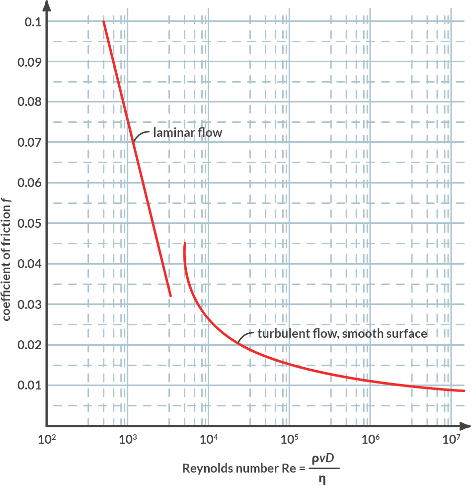
Fig. 3.13 Moody diagram.#
Pipe with height difference (continued)
In Example 3 the friction in the pipe is neglected. We assume that the total length of the pipe is 6 m and that the diameter of the pipe is 1.1 mm (which corresponds to an outflow area of 1 mm\(^2\)). Given is the density of water \(\rho = 1000\ \textrm{kg/m}^3\), and the dynamic viscosity of water, \(\eta = 1 \cdot 10^{-3}\ \textrm{Ns/m}^2\). Then calculate the force that is required to achieve the desired spray rate.
To determine whether the flow is turbulent or laminar, we first determine the Reynolds number:
The flow is turbulent (Re > 2100). From Fig. 3.13 we can see that the friction factor \(f\) is approximately 0.044. Instead of expression (3.14) we can then write:
That makes quite a difference with the original outcome! By far the largest part of the force is needed to overcome the wall friction losses.
Hydroelectric station
Using the Bernoulli equation, we can also estimate how much power the hydroelectric station in the Hoover dam can generate (Fig. 3.14 a and b).
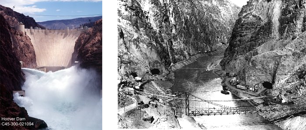
Fig. 3.14 (a) De hydroelectric station in the Hoover dam, (b) the canyon before the construction of the hydroelectric plant.#
The starting point for our estimate is the diagram from Fig. 3.14 of the plant. The water first falls over a height of 180 m. After arriving at the bottom it flows through 4 pipes, each 358 m long. Then each line divides into four. The 16 lines of 110 m eventually lead to so-called Francis turbines, which convert the movement of the water into rotational energy, which is converted into electricity by generators.
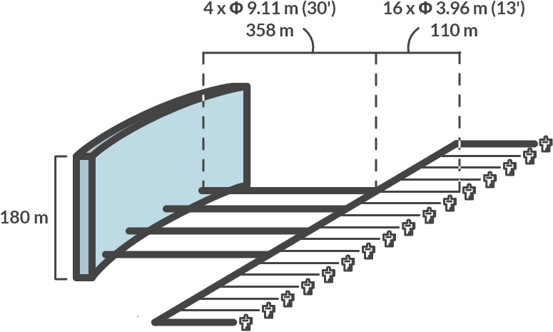
Fig. 3.15 Schematic of the Hoover dam installation.#
Furthermore, it is known (from the website) that the total volume flow through the power station can be up to \(\phi_{V,tot} = 1274\ [\textrm{m}^3/\textrm{s}]\).
Calculate the total pressure loss of the running water over the pipes that run from the Hoover dam to the turbines.
Solution
The volume flow through each of the four supply lines is \(\phi_{V1} = 1274/4 = 319\, \textrm{m}^3/\textrm{s}\)
The flow-through area of the first pipes is equal to: \(A_1 = \pi D^2/4 = 4(9.11)^2/\pi = 65.2\, \textrm{m}^2\).
The average velocity in this section \(v_1 = \phi_{V1}/A_1 = 319/65.2 = 4.9\, \textrm{ m/s}\).
The Reynolds number becomes:
We are thus on the far right of Fig. 3.13 (turbulent); the friction factor is then almost constant with a value of 0.008. The pressure loss over these pipes becomes:
This same approach can be used for the thinner pipes to the turbines:
The total pressure loss over the pipes thus becomes \((3.7 + 4.7) \cdot 10^3 = 8.4 \cdot 10^3\, \textrm{Pa} \; (1\, \textrm{Pa } = 0.084\, \textrm{bar})\) per streamline.
Calculate the dynamic pressure available for the turbines. Calculate the power that the station can deliver. The hydrodynamic power can be calculated with \(P = \Delta p \cdot \phi_V\).
Solution
The figure below shows a streamline that runs from the lake at the top of the Hoover dam, to the turbine in the power station:
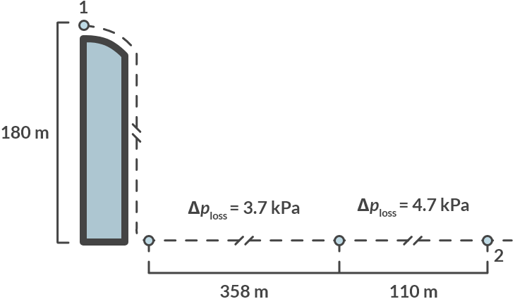
Fig. 3.16 Streamline from the Hoover dam to the turbine.#
We define points 1 and 2 on the streamline:
For point 1 we assume that \(p_1 = p_{\textrm{atmosphere}}, v_1 = 0 \quad \textrm{m/s}\) and \(h_1 = 180 \, \textrm{m}\).
For point 2 we assume that \(p_2 = p_{\textrm{atmosphere}}, v_2 = v \quad \textrm{m/s}\) and \(h_1 = 0 \, \textrm{m}\).
We also include the pressure losses that we have calculated under a.
Assuming that this dynamic pressure of \(1.76 \cdot 10^6 \, \textrm{Pa}\) is fully converted into electricity; the plant can deliver: \(P = \Delta p \phi_V = 1.76 \cdot 10^6 \cdot 1274 = 2.25 \, \textrm{GW}\).
How much power is lost to friction? Calculate the efficiency.
Solution
Friction causes a pressure loss of \(8.4 \cdot 10^3\, \textrm{Pa}\). This means that friction in the pipes \(P = \Delta p \cdot \phi_V = 8400 \times 1274 = 10.7\, \textrm{MW}\) of frictional heat. The efficiency in the transport system is then (\(2.25 \cdot 10^9 – 10.7 \cdot 10^6) / 2.25 \cdot 10^9 = 0.995 = 99.5\, \%\).
Note
Due to the numerical values of the Moody diagram, it is not possible to work parametrically here.
3.4. Fluid machines#
Due to flow losses, the pressure in a flowing medium slowly decreases, but the pressure can also be increased by adding energy. You can add energy to a flow, for example with a pump or a compressor. Due to the rotating movement of the pump, liquid is propelled and there is an increase in pressure over the pump. The added pressure through the pump is then \(\Delta p_{\textrm{pump}} = p_3 - p_4\) in which \(p_3\) is the pressure after the pump and \(p_4\) before the pump. The energy conservation comparison of a piping system with a flow machine is then equal to (3.17), the term \(\Delta p_{\textrm{pump}}\) then being added as a positive term on the left-hand side. The power that is added to the flow is then equal to \(P = \Delta p \cdot \Phi_v\) where \(\Phi_v\) is the volume flow that is shifted by the pump. In this way, mechanical energy from the pump (or ultimately perhaps electrical energy if it concerns an electric pump) becomes potential energy from the flow. The mechanical (or electrical) power that the pump uses is usually significantly larger than the power \(P = \Delta p \cdot \Phi_v\) absorbed by the flow. This is due to losses, so that the efficiency of the pump is less than 100%. The impeller of the pump also creates swirls and turbulence that are eventually dissipated and transferred to heat (that heat increase is usually small). Designing the correct geometry of a pump is therefore very important and a subject that plays an important role in mechanical engineering.
Not only can energy be added to a flow, energy can also be extracted, as can be seen for example in Example Hydroelectric station of the hydroelectric station. Energy is often extracted by a fan that is driven by the current, such as a windmill or a turbine. A turbine is similar to a pump, but the energy is now added to the flow. Now a pressure loss term must be added to (3.17) as a loss term so the term \(- \Delta p_{\textrm{turbine}}\) is added to the left-hand side.
Note
The minus sign indicates that energy is extracted. The design of the correct form of blades for a windmill or a turbine is also an important subject in mechanical engineering.
3.5. What lies ahead#
In this chapter you have become acquainted with the fields of liquids and flow. The theory in the field of flow can still be considerably expanded. In fact, the theory needs to be expanded further because a turbulent flow is still not fully understood. Einstein called this the last unsolved problem in physics.
For the design process of these devices, it is necessary to have insight into both the small-scale physical phenomena that play a role and the relationship between the device and the other parts of the installation. Flow analysis leans against the field of physical transport phenomena from physics.
In practice, flow devices for the compression and expansion of liquids and gases are often used in combinations with all kinds of other processes and devices, for example reactors (process devices), combustion for power generation (e.g. in an engine or gas turbine), or phase transitions (e.g. in separation devices). Heat machines, in which the heat is added or extracted from the liquid, are already discussed in the next chapter. In the mechanical engineering curriculum you also receive various follow-up courses that continue with this topic.
3.6. Problems#
Even though the questions are formulated in a compact manner, a complete calculation with explanation is requested. Start with the basic equations. Apply them subsequently to the specific situation. Try to work parametrically as long as possible using symbols only. Substitute the numerical values only at the end. Give the final value with an appropriate number of significant digits and the correct unit.
Since in this chapter it is mainly about the solution method and not the exact value of the answer, we will use the following approximate values:
Gravitation acceleration \(g = 10 \textrm{ m}/\textrm{s}^2\)
Atmospheric pressure \(p_0 = 1.0\textrm{ bar} = 1.0\cdot 10^5 \textrm{ Pa}\)
Density of water \(\rho = 1 \cdot 10^3 \textrm{ kg}/\textrm{m}^3\)
Viscosity of water \(\eta = 1.0\cdot 10^{-3} \textrm{ Pa}\textrm{ s}\)
Exercise 3.1 (Water tank with hose)
In a water tank with a diameter Ø of \(600\) mm the water level is \(3.0\) m high. In the bottom, a hole of Ø 20 mm is drilled, see Figure 6.1.
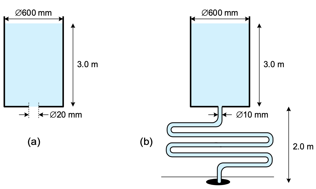
Fig. 3.17 Tank with hole in the bottom (left), tank with 20 m long hose (right).#
Calculate the outflow velocity of the water when friction is neglected. Compare your answer with the velocity of a free-falling object.
A mechanic manages to connect a hose with inner diameter Ø \(10\) mm leak free to the bottom of the tank. The hose is \(20\) m long and ends up in a drain \(2.0\) m below the bottom of the tank.
Calculate the outflow velocity of the water into the drain, neglecting friction.
Calculate the pressure drop by friction in the hose when the water flows out of the hose with a velocity \(1.0 \textrm{ m}/\textrm{s}\).
Tip
First use the Reynolds number to determine whether the flow is laminar or turbulent.
Show that, due to friction in the hose, the outflow velocity becomes \(1.374 \textrm{ m}/\textrm{s}\) (when no external forces are exerted on the system).
Note that if friction losses are included, the outflow velocity cannot be easily found.
Exercise 3.2 (Solar water heating with closed return-system)
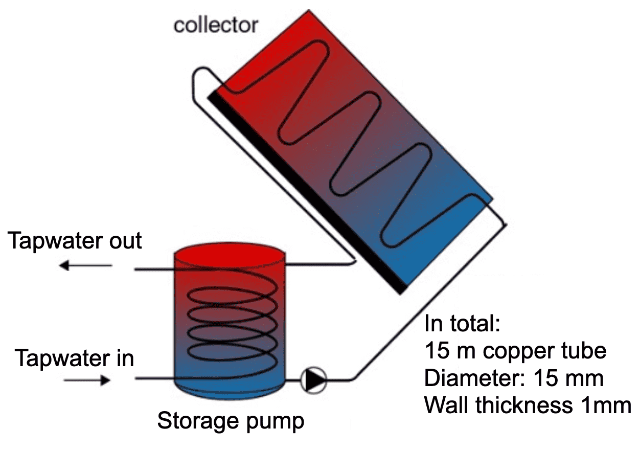
Fig. 3.18 Schematic view of the solar collector.#
Fig. 3.18 depicts a schematic view of the solar collector system that we will analyze critically. The system is closed. If there would be no friction, and the tube would be completely filled, then the pump would not have to deliver power. Unfortunately, in reality there is friction of course.
The friction losses correspond to the friction of a \(15\) m long copper pipe with an outer diameter of \(15\) mm and a wall thickness of \(1\) mm. The system is filled with water.
The flow rate of water through the collector is \(6\) liter\(/\)min.
Determine whether the flow is laminar or turbulent.
Tip
Calculate the velocity of the water in the tube.
Calculate the pressure drop per meter due to friction in the tube.
Calculate the power that the pump has to deliver.
Indeed, the required power is very low. Usually, circulation pumps of central heating systems are used for this purpose. The smallest commercially available pump has a power of about \(20\) W, which is already much too powerful.
Exercise 3.3 (Self-draining solar water heating system)
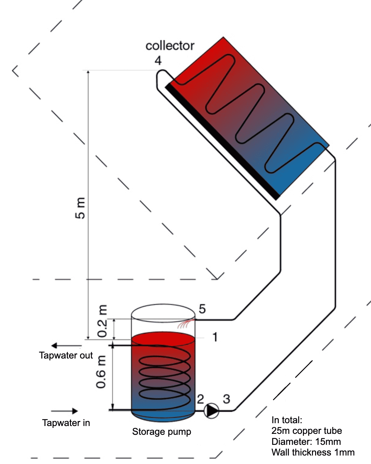
Fig. 3.19 Schematic representation of the solar heater with self-draining system.#
A decade ago, whole neighborhoods in the Netherlands were equipped with solar water heaters. The collectors were usually mounted on the roof and the storage tanks in the attic. In the winter that followed after the installation, all these collectors froze.
In order to prevent this, the system can be changed into a self-draining system, see Fig. 3.19. The storage tank is now placed \(5\) m lower and is open to the surrounding. The volume of the tank is much bigger than the volume of the rest of the system. The pump is connected to the tank with a small pipe. When the pump is shut down, the water flows out of the collector to the tank and the lower located tubes.
Explain why the storage tank is placed below the collector. Does the same reason apply to the collector of Fig. 3.18 from the previous exercise?
In order to start the system, the pump has to pump the water to the highest point. After that, the water will flow through the return pipe back to the tank. The return pipe ends \(20\) cm above the water surface. The velocity at which the system is filled, is not very important: You may assume that it is very low.
A streamline with 5 points is defined, see Fig. 3.19. It is assumed that the fluid velocity in all these points is the same, but \(v_1 = 0 \textrm{ m}/\textrm{s}\) (why?)
The water flow rate through the collector remains \(6 \textrm{ liter}/\textrm{min}\) (as in Exercise 3.2).
Calculate the pressure \(p_2\), just before the pump (in point \(2\)) during filling.
Calculate the pressure \(p_3\), just after the pump (in point 3) during filling, when the water column has exactly reached the highest point \(4\) and the return pipe is still empty
Calculate the pressure the pump has to deliver to start the system.
Calculate the pressure the pump has to deliver when the system is in normal operation and friction losses can be ignored. In normal operation the whole tube (from point \(1\) to \(5\)) is filled with water.
Calculate the pressure the pump has to deliver when the system is in normal operation and friction losses are included.
Calculate the power the pump has to deliver to start the system, and in normal operation.
What can you conclude about the choice of pump, regarding the required pressure and power (for starting and normal operation)?
Exercise 3.4 (Tubing of a cooling system)
In Figure 6.4 a schematic diagram of an engine cooling system is shown. At the left, an engine block transfers its heat (see arrow direction) to the cooling tube and at the right (a part of) the heat leaves the system through the radiator. The coolant (\(\rho = 1100 \textrm{ kg}/\textrm{m}^3,\, \eta = 4.5\cdot 10^{-4}\, \textrm{ Pa} \textrm{s},\; c = 5000 \textrm{ J}/\textrm{kg K}\)) has a mass flow rate of \(0.22 \textrm{ kg}/\textrm{s}\). We approximate the cooling system as a closed tubing system with bends, as depicted in Fig. 3.20. The tube of the cooling system has an inner diameter of Ø \(15\) mm.
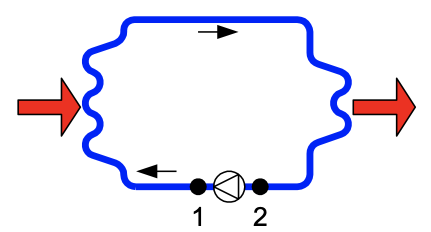
Fig. 3.20 Schematic diagram of the cooling system indicating points 1 and 2.#
Calculate the velocity at which the coolant flows through the tube.
The length of the cooling tube is \(4.0\) meter. The bends in the tube cause extra pressure losses. The pressure loss \(\Delta p_{\textrm{loss}}\) of the tube and bends together is given by
Parameters |
|
|---|---|
\(f\) |
Friction factor [-] |
\(L\) |
Tube length in [m] |
\(D\) |
Tube diameter in [m] |
\(\rho\) |
Density of the medium in [\(\textrm{kg}/ \textrm{m}^3\)] |
\(v\) |
Flow velocity in [\(\textrm{m}/\textrm{s}\)] |
The extra term of \(12.5\) in the equation above represents the pressure loss due to the bends in the system.
Write down Bernouilli’s equation for the system with point \(1\) just after the pump and point \(2\) just before the pump, as depicted in Fig. 3.20.
Calculate the pressure difference the pump has to deliver to reach the desired flow velocity.
Calculate the power that the pump has to deliver.
Exercise 3.5 (Cooling of a surface via flows in cooling channels)
In a wafer stepper as used in semiconductor lithography, the reticle (also called a photomask) contains the microscopic circuit pattern that is projected onto the wafer using extreme ultraviolet (EUV) or deep ultraviolet (DUV) light. Because the reticle is directly exposed to intense radiation, part of the light energy is absorbed and converted into heat. This heating can cause:
Thermal expansion of the reticle, leading to distortion of the projected pattern.
Loss of alignment accuracy, since even nanometer-scale deformation can ruin chip quality.
Reduced lifetime of the reticle if overheating is not controlled.
To prevent these problems, reticle cooling is implemented:
The reticle is mounted in a reticle clamp or chuck that has integrated micro cooling channels.
A cooling fluid (usually water, kept ultra-clean to avoid contamination) flows through these channels.
Heat absorbed from EUV/DUV light is conducted away through the clamp into the coolant.
In Fig. 3.21 below one of these rectile cooling systems is visible.
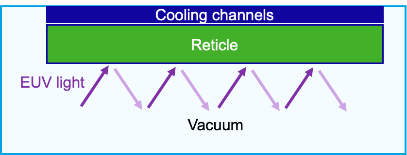
Fig. 3.21 Schematic cross-sectional view of the reticle cooling setup, showing the reticle clamped under cooling channels, with EUV light passing through and reflecting in vacuum.#
The reticle contains the pattern that needs to be imaged at the wafer. The EUV light that is used for imaging is partially absorbed by the reticle. To avoid excessive thermal expansion, the reticle clamp is equipped with cooling channels. The width of the reticle is equal to \(W = 104 \cdot 10^{-3} \, [\textrm{m}]\) and its length equal to \(L = 132 \cdot 10^{-3} \, [\textrm{m}]\). The diameter of the inlet is equal to \(D_i = 40 \cdot 10^{-3} \, [\textrm{m}]\) and those of the cooling channels equal to \(D_c = 20 \cdot 10^{-3} \, [\textrm{m}]\). The top view of this system may be see in Fig. 3.22 below.
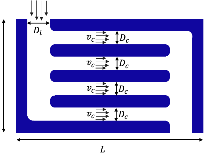
Fig. 3.22 Top view of the reticle cooling channels, illustrating the inlet diameter \(D_i\), flow velocity \(v_i\), cooling channel diameter \(D_c\), flow velocity \(v_c\), reticle width \(W\), and length \(L\).#
Suppose the flow of the inlet is equal to \(3 \, \textrm{liter/min}\). To avoid flow-induced vibrations, the flow must be laminar. What is the Reynolds number in the inlet and the cooling channels?
What is the pressure drop over the cooling channels (when neglecting the pressure drop over the inlet)?
Now suppose the reticle requires more cooling so the inlet flow is increased to \(5 \, \textrm{liter/min}\). What is the impact? How does the design need to be changed?